Convolution of waveforms using Python compared to MATLAB

We will see compare the convolution functions in Python (Numpy or Scipy) with the conv function in MATLAB. If you have tried them both then you would know that its not exactly same. In the end we will try to find how can we make the Python convolution works in the same way as the MATLAB one. This can be helpful in translating the code from MATLAB to Python.

Convolution

Convolution is a mathematical operation on two functions (\(f\) and \(g\)) that produces a third function \( conv \) that expresses how the shape of one is modified by the other. It is defined as the integral of the product of the two functions after one is reversed and shifted.

\begin{equation} f * g (t) = \int_{-\infty}^{\infty} f(\tau) g(t-\tau) d\tau \end{equation}

We have seen several posts about the cross-correlation. Convolution can be seen as the cross-correlation of \(f(x)\) and \(g(-x)\), or \(f(-x)\) and \(g(x)\) for the real-valued functions. For the complex valued functions, the cross-correlation operator is the adjoint of the convolution operator.

1-D convolution analytical example

Let us take two arrays:

f = [1, 2, 3]
g = [5, 6, 7]

Now, let us compute the convolution of the two arrays step by step:

1. Reverse the function \(g\) for the \(f*g\).

   f = [1, 2, 3]
   g_ = [7, 6, 5]
   

2. Now, we compute the convolution at t = 0

   f = [_, _, 1, 2, 3]
   g_ = [7, 6, 5, 0, 0]
   prod0 = [_, _, 5, 0, 0] = 5
   

3. Then, we compute the convolution at t = 1

   f = [_, 1, 2, 3]
   g_ = [7, 6, 5, 0]
   prod1 = [_, 6, 10, 0] = 16
   

4. Then, we compute the convolution at t = 2

   f = [1, 2, 3]
   g_ = [7, 6, 5]
   prod2 = [7, 12, 15] = 34
   

5. Then, we compute the convolution at t = 3

   f = [1, 2, 3, _]
   g_ = [0, 7, 6, 5]
   prod3 = [0, 14, 18, _] = 32
   

6. Then, we compute the convolution at t = 4

   f = [1, 2, 3, _]
   g_ = [_, 0, 7, 6]
   prod3 = [_, 0, 21, _] = 21
   

So, we got the convolution to be: [5, 16, 34, 32, 21].

Convolution using Python

Using the mode full

Python

import numpy as np

f = [1, 2, 3]
g = [5, 6, 7]

conv1 = np.convolve(f,g,'full')

print(conv1)

$ [ 5 16 34 32 21]

MATLAB

clear all; close all; clc;

f = [1 2 3];
g = [5 6 7];

fgconv = conv(f,g,'full')

fgconv =

     5    16    34    32    21

Using the mode same

This returns the output of the length same as the max(len(f), len(g)).

Python

import numpy as np

f = [1, 2, 3]
g = [5, 6, 7]

conv1 = np.convolve(f,g,'same')

print(conv1)

$ [16 34 32]

MATLAB

clear all; close all; clc;

f = [1 2 3];
g = [5 6 7];

fgconv = conv(f,g,'same')

fgconv =

    16    34    32

Using the mode valid

The convolution product is only given for points where the signals overlap completely.

Python

import numpy as np

f = [1, 2, 3]
g = [5, 6, 7]

conv1 = np.convolve(f,g,'valid')

print(conv1)

$ [34]

MATLAB

clear all; close all; clc;

f = [1 2 3];
g = [5 6 7];

fgconv = conv(f,g,'valid')

fgconv =

    34

Convolution of signals of different lengths

Now, let us consider a case where the length of the two arrays differs for the mode same. It is as we can expect, same for the full and valid mode. Let us first compute the covolution in Python using the same approach.

Python

import numpy as np

f = [-1, 2, 3, -2, 0, 1, 2]
g = [2, 4, -1, 1]

conv1 = np.convolve(f,g,'same')
print(conv1)

$ [ 0 15  5 -9  7  6  7]

MATLAB

clear all; close all; clc;

f = [-1 2 3 -2 0 1 2];
g = [2 4 -1 1];

fgconv = conv(f,g,'same')

fgconv =

    15     5    -9     7     6     7    -1

This post explains the reason behind this.

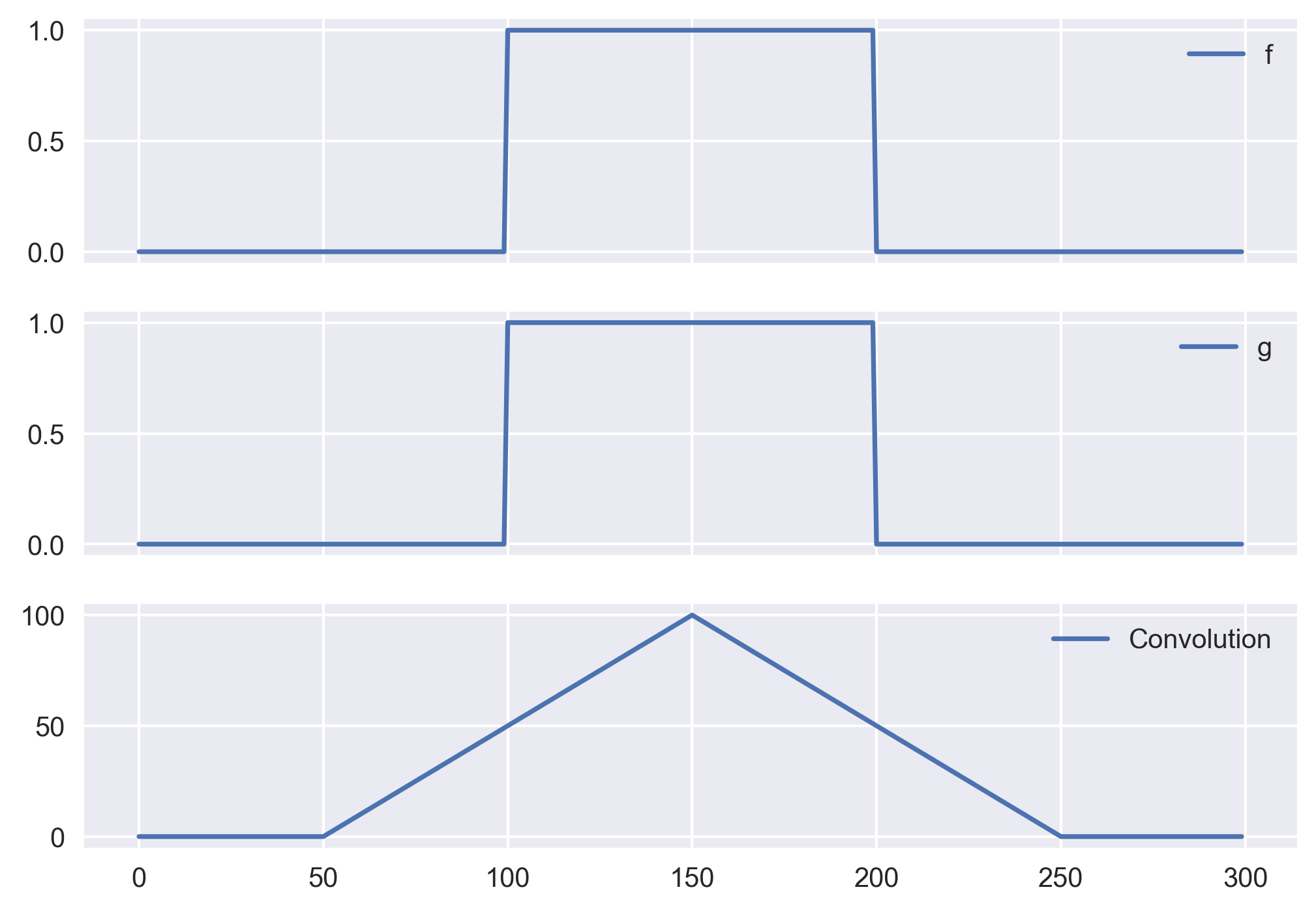
Convolution of two signals

Let us take two heaviside functions and compute the convolution of the two. Note that in this case, the convolution is same as the correlation because the function g is even function (\(g(\tau) = g(-\tau)\)).

import numpy as np
from scipy import signal
import matplotlib.pyplot as plt
plt.style.use('seaborn')

sig1 = np.repeat([0., 1., 0.], 100)
sig2 = np.repeat([0., 1., 0.], 100)

filtered = np.convolve(sig1, sig2, mode='same')

fig, ax = plt.subplots(3,1, sharex=True)
ax[0].plot(sig1, label='f')
ax[1].plot(sig2, label='g')
ax[2].plot(filtered, label = 'Convolution')

for axx in ax:
    axx.legend()

plt.savefig('convolvesigs.png',bbox_inches='tight', dpi=300)

Conclusions

So, we can conclude that the Python and MATLAB implementation of the convolution function results same output when the length of the two arrays is same. However, when the length of the two arrays is not same, then the way MATLAB does the padding is slightly different than that of Python for the mode where we output the arrays of the same length as the minimum length of the arrays.