
Concatenating daily seismic traces into one MiniSeed File (codes included)
I concatenate the daily seismic traces for 15 days into one miniseed file for further analysis. Then I obtained the spectrogram of the 15 days seismic data. Codes included.
I have daily seismic traces for several days. I need to concatenate them into one for analysis. This post will show you how you can use Obspy to achieve that. Following is the list of steps to achieve that.
Import necessary libraries
First step is to import necessary libraries.
import glob, os
import numpy as np
import matplotlib.pyplot as plt
plt.rcParams['figure.figsize'] = [10,6]
plt.rcParams.update({'font.size': 18})
plt.style.use('seaborn')
from obspy import read, Stream
I will use the glob and os to find the data files, read to read the mseed file into memory. Stream will be used to create a new obspy “stream” object for the final concatenated mseed file.
Similar posts
Concatenate the traces
In the below script snippet, mseed_data is the list of all the mseed file paths, datarange is the indexes of the files that will be concatenated. Please note that if your file paths are not sorted then you will have to sort it first. I loop through each of the 15 files and append it to the mytrace object iteratively.
mseed_data = glob.glob(os.path.join("data", "*.mseed"))
downsample = True
datarange = np.arange(0,15, dtype=int)
stZ = read(mseed_data[datarange[0]])
mytrace = stZ[0]

starttime0 = mytrace.stats.starttime
endtime0 = mytrace.stats.endtime

for i,trdata in enumerate(mseed_data[datarange[1]:datarange[-1]]):
    st = read(trdata)
    if i==0:
        oldend = endtime0
    print(f"Reading trace {i+2}: {trdata}, range: {st[0].stats.starttime}-{st[0].stats.endtime}, jump: {st[0].stats.starttime-oldend} second")
    tr = st[0]

    mytrace+=tr
    oldend = tr.stats.endtime

mystream = Stream(traces=[mytrace])
for tr in mystream:
    if isinstance(tr.data, np.ma.masked_array):
        tr.data = tr.data.filled(0)

if downsample:
  ## I want the final sampling rate to be 1Hz
  mystream.interpolate(sampling_rate=mystream[0].stats.sampling_rate/mystream[0].stats.sampling_rate,starttime=starttime0) #to deal with missing data

  #abort downsampling in case of changing end times (strict_length=true)
  # mystream[0].decimate(factor=10, strict_length=False, no_filter=False) #lowpass filter is applied to ensure no aliasing artifacts are introduced
  # mystream[0].decimate(factor=4, strict_length=False, no_filter=False)

mystream.write(mseed_data_comb, format="MSEED")
Finally, the missing values are masked by filling the 0s. Sometimes, you would like to downsample the traces for the further analysis. My traces are 40 Hz originally, and I downsampled it to 1Hz (1 samples/second). Please note that the above script shows two ways of downsampling - interpolation, or decimate. You can select either one based on your needs.
Finally, I wrote the stream into a mseed file.
Plot the traces
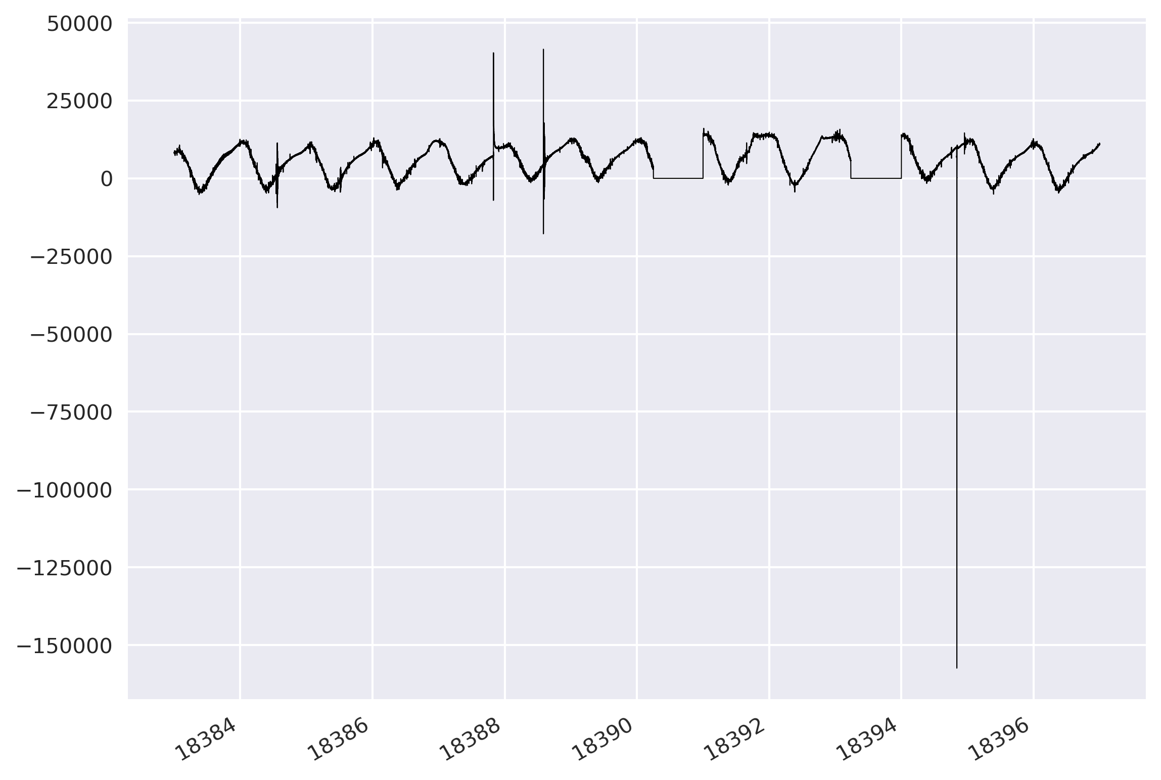
I read the concatenated mseed file and plotted its data with respect to its time.
newMseed = read(mseed_data_comb)
print(newMseed)
fig, ax = plt.subplots(1,1)
ax.plot(newMseed[0].times('matplotlib'), newMseed[0].data, lw=0.5, color='k')

fig.autofmt_xdate()
plt.tight_layout()
plt.savefig('new-mseed-data.png', bbox_inches='tight', dpi=300)
plt.close('all')
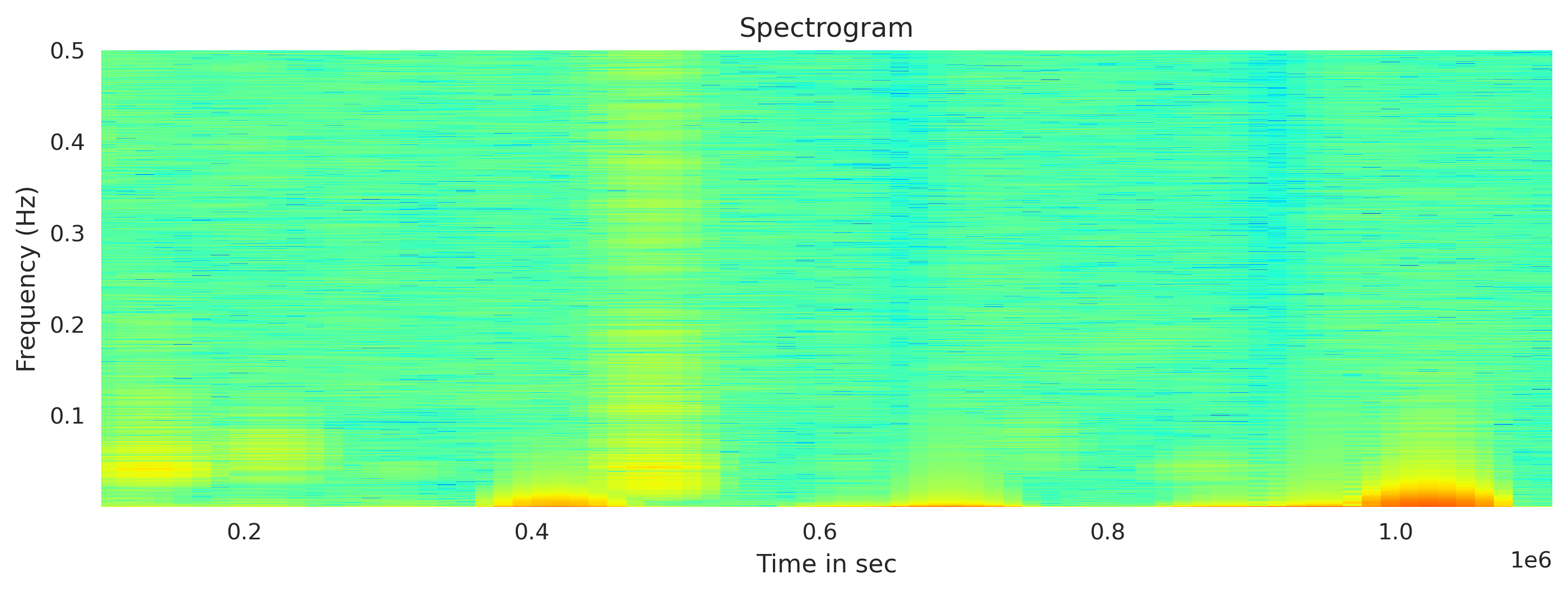
Plot the spectrogram using Obspy
For the fft window length, I used the 12th of the total length of the traces (arbitrarily). The output amplitude is in the dbscale. I clip the x axis to show the obtained values only (remove the masked values)
## Plot spectrogram
fig, axx = plt.subplots(1,1, figsize=(10,4))
total_length = newMseed[0].data.shape[0]
wlength = int(total_length/12) #window length for fft
newMseed[0].spectrogram(log=True, wlen=wlength,show=False, axes=axx, cmap='jet', dbscale=True) #wlen for the trade off between freq and time
ymin, ymax = axx.get_ylim()
xmin, xmax = axx.get_xlim()

print(xmin, xmax, ymin, ymax)
axx.set_xlim([xmin+wlength, xmax-wlength])
axx.set_title('Spectrogram')
axx.set_xlabel('Time in sec')
axx.set_ylabel('Frequency (Hz)')
plt.tight_layout()
plt.savefig('spectrogram_plot.png', bbox_inches='tight', dpi=300)
plt.close('all')
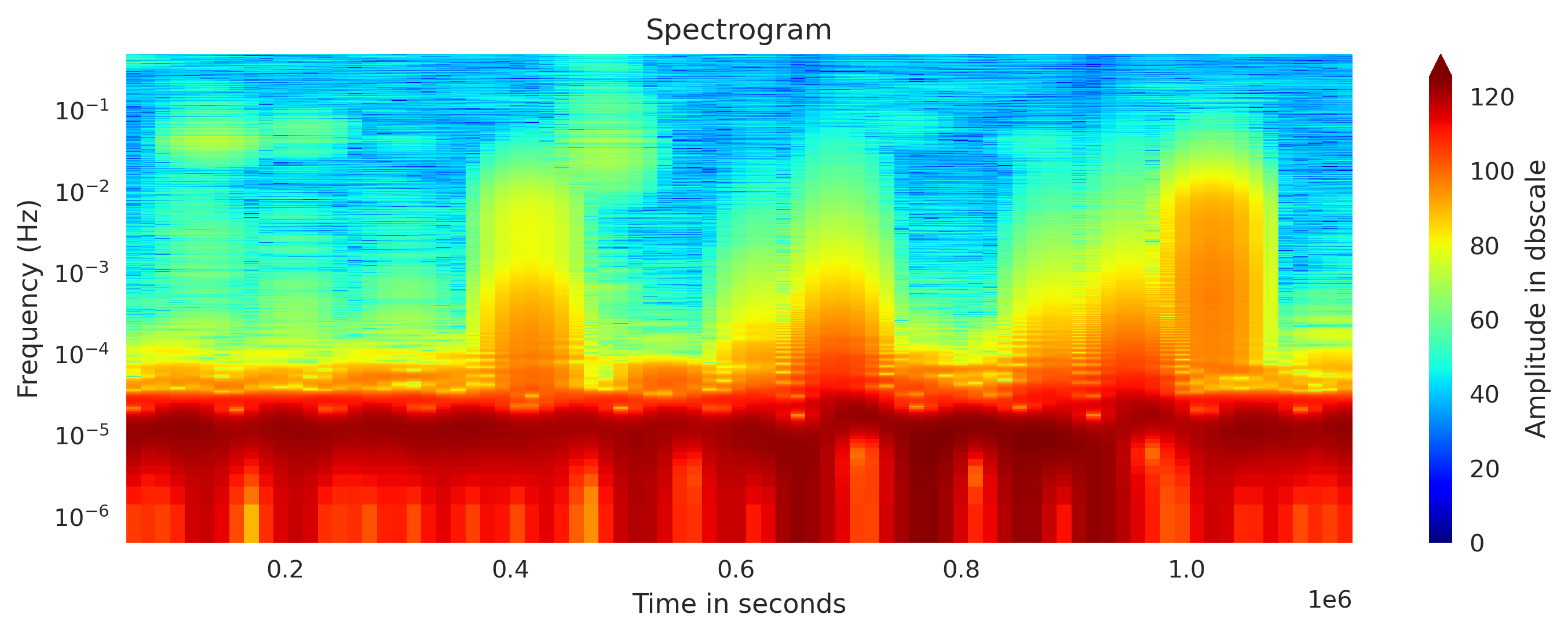
Plot custom spectrogram
I modfied the Obspy’s spectrogram function to obtain the spectrogram computation results and then I plotted it. This provides us more control on the plotting and customization.
from matplotlib.colors import Normalize
from spectrogram_obspy_modified import compute_spectrogram

## Plot spectrogram
fig, axx = plt.subplots(1,1, figsize=(10,4))
total_length = newMseed[0].data.shape[0]
wlength = int(total_length/12) #window length for fft

specgram, freq, time = compute_spectrogram(newMseed[0].data,samp_rate=newMseed[0].stats.sampling_rate, wlen=wlength, dbscale=True) #wlen for the trade off between freq and time

## Normalize the color map
vmin = specgram.min()
vmax = specgram.max()
if vmin<0:
    vmin = 0
norm = Normalize(vmin, vmax, clip=True)
axx.set_yscale('log')
cscale = axx.pcolormesh(time, freq, specgram, norm=norm, cmap='jet')
# Log scaling for frequency values (y-axis)

axx.set_title('Spectrogram')
axx.set_xlabel('Time in seconds')
axx.set_ylabel('Frequency (Hz)')
cbar = fig.colorbar(cscale, extend='max')
cbar.set_label('Amplitude in dbscale')
plt.tight_layout()
plt.savefig('spectrogram_plot2.png', bbox_inches='tight', dpi=300)
plt.close('all')
The modified script can be downloaded from here.
The complete script for this post can be downloaded from here.
Disclaimer of liability
The information provided by the Earth Inversion is made available for educational purposes only.
Whilst we endeavor to keep the information up-to-date and correct. Earth Inversion makes no representations or warranties of any kind, express or implied about the completeness, accuracy, reliability, suitability or availability with respect to the website or the information, products, services or related graphics content on the website for any purpose.
UNDER NO CIRCUMSTANCE SHALL WE HAVE ANY LIABILITY TO YOU FOR ANY LOSS OR DAMAGE OF ANY KIND INCURRED AS A RESULT OF THE USE OF THE SITE OR RELIANCE ON ANY INFORMATION PROVIDED ON THE SITE. ANY RELIANCE YOU PLACED ON SUCH MATERIAL IS THEREFORE STRICTLY AT YOUR OWN RISK.
Leave a comment