Time Series Analysis in Geophysics (codes included)

Time-series analysis is essential in most fields of science, including geophysics, economics, etc. Most of the geophysical data comes in a time-series format, including the seismic recordings. In this part of the series of tutorial, we will see how we can quickly load the data, and visualize it.

Prerequisites

This tutorial does not require the reader to have any basic understanding of Python or any programming language. But we expect the reader to have installed the jupyter notebook on their system. If the reader has not installed it yet, then they can follow the previous post where we went through the steps involved in getting started with Python.

What is Time-series?

Time-series is a collection of data at fixed time intervals. This can be analyzed to obtain long-term trends, statistics, and many other sorts of inferences depending on the subject.

Data

We also need some data to undergo the analysis. We demonstrate the analysis using our GPS data. It can be downloaded from here.

No access to the sample file? The .COR file is just whitespace-separated columns (Year, Lat, Long, Hgt, dN, dE, dU), so the workflow below works on any such table — point pd.read_csv(...) at your own GPS/geodetic time series (or any CSV) and rename the columns to match.

Let’s get started

The first step is always to start the Python interpreter. In our case, we will use the jupyter notebook.

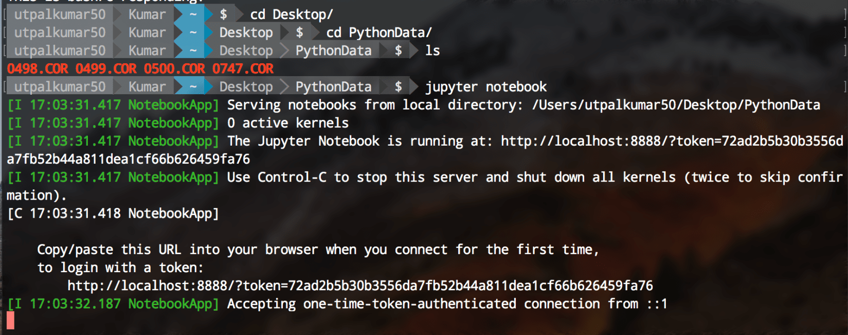
Jupyter notebook can be started using the terminal. Firstly, navigate to your directory containing the data and the type “jupyter notebook” on your terminal.

jupyter notebook

Next, we create a new Python 3 notebook, rename it as pythontut1. Then, we need to import some of the libraries:

import pandas as pd
import numpy as np
import matplotlib.pyplot as plt
%matplotlib inline
from matplotlib.pyplot import rcParams
rcParams['figure.figsize'] = 15, 6

Loading the data

Now, we load the data using the pandas library functions. Here, we use the function read_csv. But, before that let’s observe the format of the data:

!head 0498.COR

The prefix “!” can be used to execute any Linux command in the notebook.

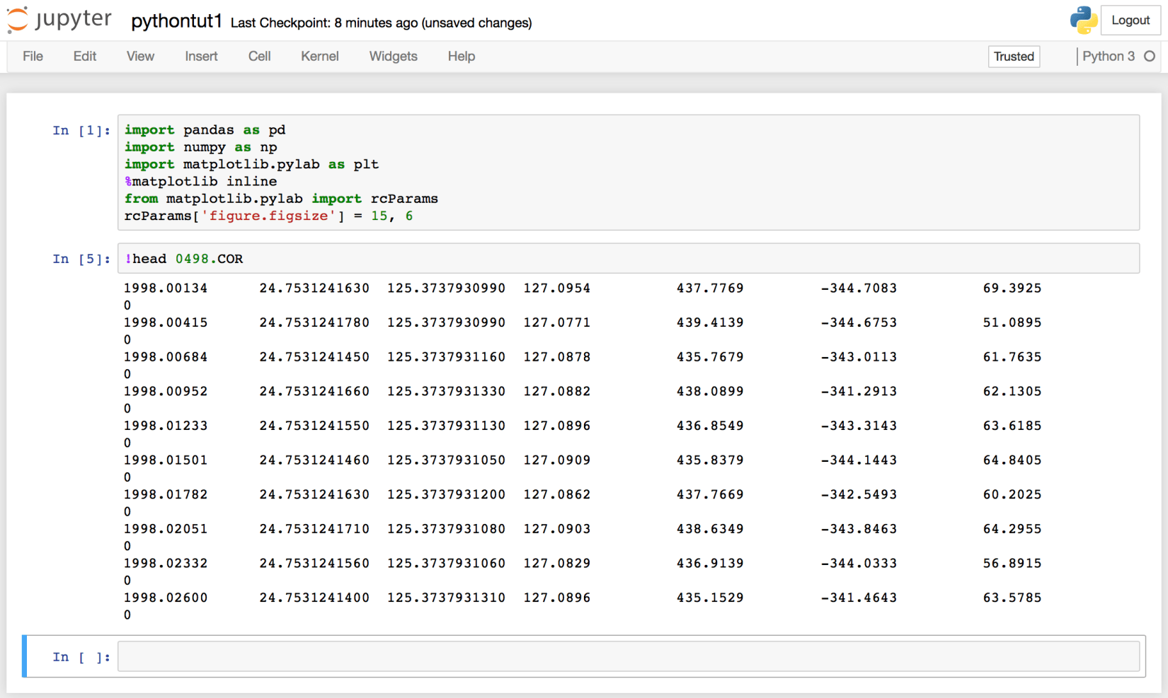
We can see that the data has no header information, and 8 columns. The columns are namely, “year”, “latitude”, “longitude”, “Height”, “dN”, “dE”, “dU”.

So, now we read the data and set the above names to the different columns.

df=pd.read_csv("0498.COR", header=None, delimiter='\s+', names=['Year',"Lat","Long","Hgt","dN","dE","dU","nav"])
df.head()

It is essential to understand the above command. We gave the argument of the filename, header (default is the first line), delimiter (default is a comma) and the names of each column, respectively. Then we output the first 5 lines of the data using the df.head() command.

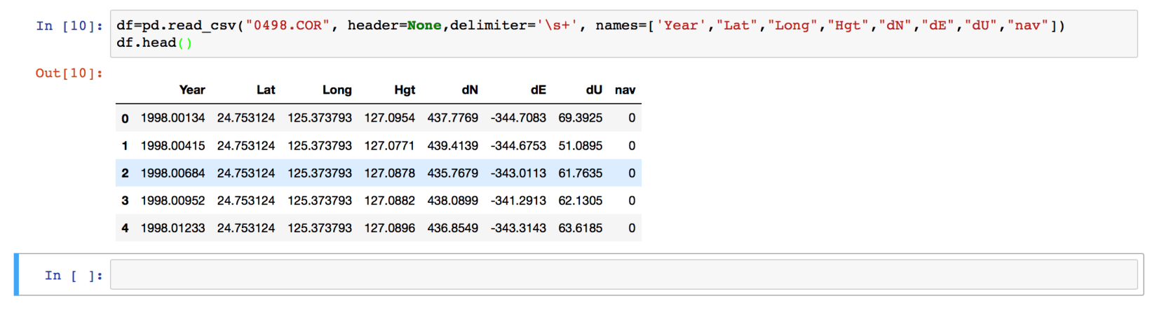
Our data is now loaded, and if we want to extract any section of the data, we can easily do that.

df['Year'].head()
df[['Year','Lat']].head()

Here, we have used the column names to extract the two columns only. We can also use the index values.

df.loc[:,"Year"].head()
df.iloc[:,3].head()

When we use “.loc” method to extract the section of the data, then we need to use the column name whereas when we use the “.iloc” method then we use the index values. Here, df.iloc[:,3] extracts all the rows of the 3rd column (“Hgt”).

Analysis

Now, we have the data loaded. Let’s plot the “dN”, “dE”, and “dU” values versus the year. Before doing that, let’s set the “Year” column as the index column.

df.set_index("Year", inplace=True)
df.head()

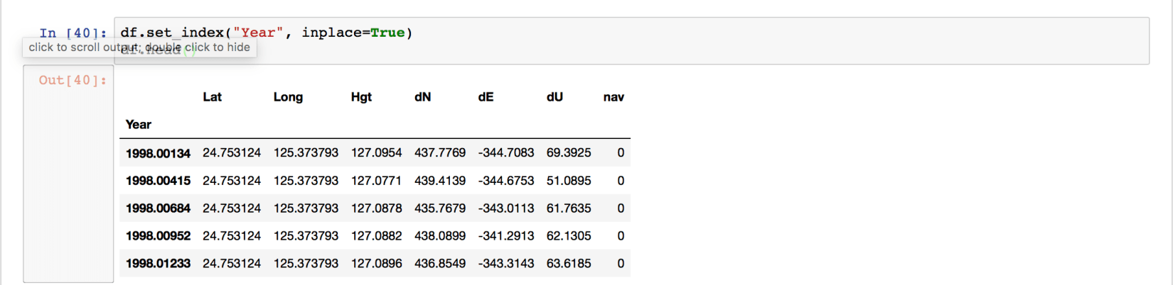
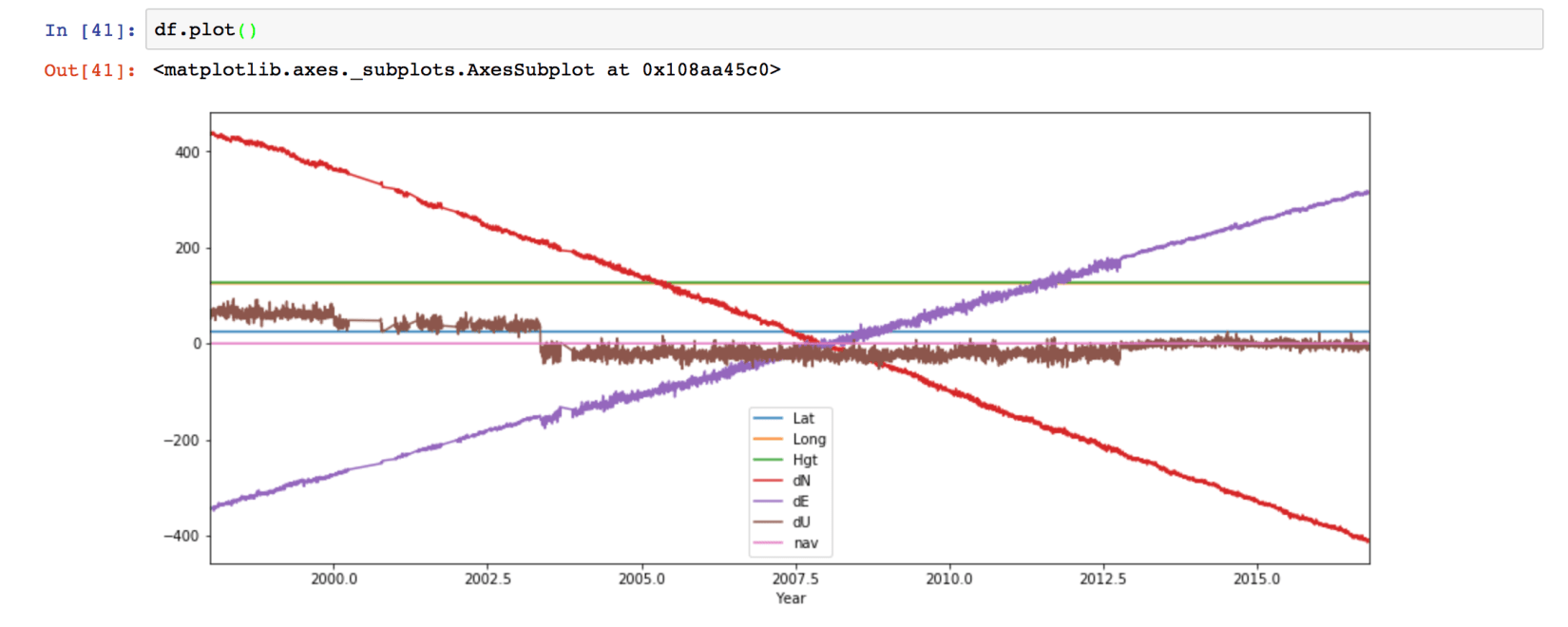
We can see the “Year” column as the index of the data frame now. Plotting using Pandas is extremely easy.

df.plot()

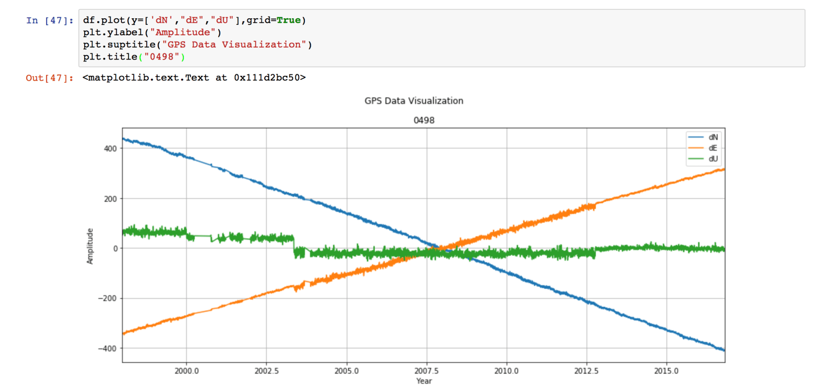
We can also customize the plot easily.

df.plot(y=['dN',"dE","dU"],grid=True)
plt.ylabel("Amplitude")
plt.suptitle("GPS Data Visualization")
plt.title("0498")

If we want to save the figure, then we can use the command:

plt.savefig('0498Data.pdf',dpi=300,bbox_inches='tight')

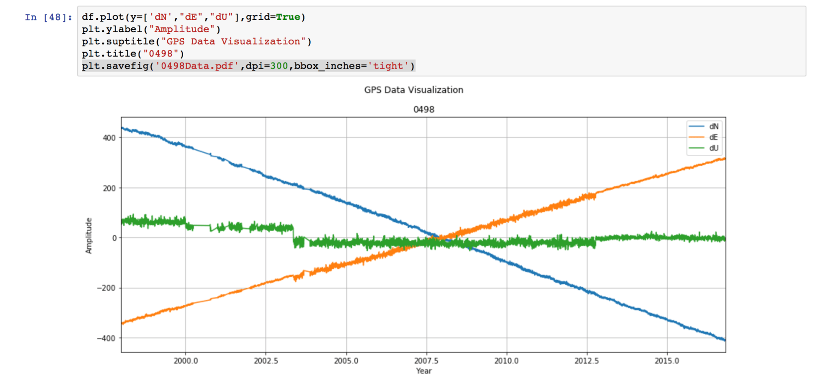
This saves the figure as the pdf file named “0498Data.pdf”. The format can be set to any type “.png”, “.jpg”, ‘.eps”, etc. We set the resolution to be 300 dpi. This can be varied depending on our need. Lastly, “bbox_inches =‘tight’” crops our figure to remove all the unnecessary space.

Next Tutorial

We have loaded the data and visualized it. But we can see that our data has some trend and seasonality. In the next tutorial we will learn how to filter and smooth the data to separate those components.

Recap

• A time series is data sampled at regular intervals; geophysical ones typically combine a trend, a seasonal/periodic part, and residual noise.
• Load whitespace-separated data with pd.read_csv(..., delimiter='\s+', names=[...]), giving the columns names since the file has no header.
• Slice with df[['col1','col2']], .loc[:, "name"] (by label), or .iloc[:, 3] (by position).
• Set the time column as the index (df.set_index("Year")) so df.plot() uses it as the x-axis automatically.
• This is step one — seeing the trend and seasonality. Removing them (detrending, filtering) comes next.

Where to go next

• Time-series analysis: filtering and smoothing data — the direct follow-up: separate trend from noise.
• How to start using pandas for Earth data analysis — deeper on the dataframe operations used here.
• Signal denoising using the Fast Fourier Transform — inspect the periodic content in the frequency domain.