Plotting a record section using Obspy (codes included)
Introduction
In this post, I will show you the steps for making a quick record section starting from a set of SAC data in the folder. The record section plot is one of the first thing seismologists like to do when we receive the data and plan to apply some methods. If you are simply interested in plotting the seismograms with distance, you may like my post:
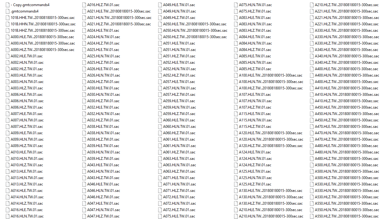
My data folder contains SAC data of different naming format (because I mixed the data from different networks). Nevertheless, we will read all of them in our program (even sort them based on vertical, north or east components) and then plot the record section. I will also show you some of the customizations you can do to make the record section visually appealing.
Key idea — a record section stacks waveforms by distance. Instead of overlaying seismograms, a record section plots each trace at a vertical position equal to its epicentral distance from the earthquake, with time along the other axis. Because a seismic wave reaches farther stations later, the first arrivals line up along a sloping moveout — and that slope is the wave’s apparent velocity. The one thing ObsPy needs to do this is the distance stored in each trace’s header: tr.stats.distance (in metres). Set that, then call stream.plot(type='section').
Using Obspy’s plot method
Obspy has a good documentation on how to plot the record section. I recommend reader to give a look to the documentation as we cannot cover all the features in this post. But I show you a special case with some customizations. It is always helpful to have several examples in our reach when we are trying to do some coding. It makes the whole process fast and efficient.
Libraries required
For this tutorial, only library we need is obspy. It comes with several dependencies including numpy, matplotlib, etc. For this section, we will only use the plot method of the Obspy’s Stream class. In the next section, I will show you how to plot the record section using the matplotlib to obtain similar results. Since, matplotlib is a lower level library so it offers more flexibility.
The obspy library can be installed simply by:
pip install obspy
Reading the data
Now, we first read the list of data using the glob module.
from obspy import read, Stream
import glob
all_z_data = glob.glob("*H?Z*-300sec.sac")
Notice that in the argument of the glob function, I used "*H?Z*-300sec.sac". This is an expression for finding all the files containing the letters H and Z and ending with the suffix -300sec.sac. There are several files in my directory that does not have similar filename formats. I want to exclude those. If you want to include all the sac files, you can simply use "*.sac".
The glob function returns a list of the all the files with the match. In my case, it returns a list of length 350. So, I have 350 SAC files that conforms to that file name.
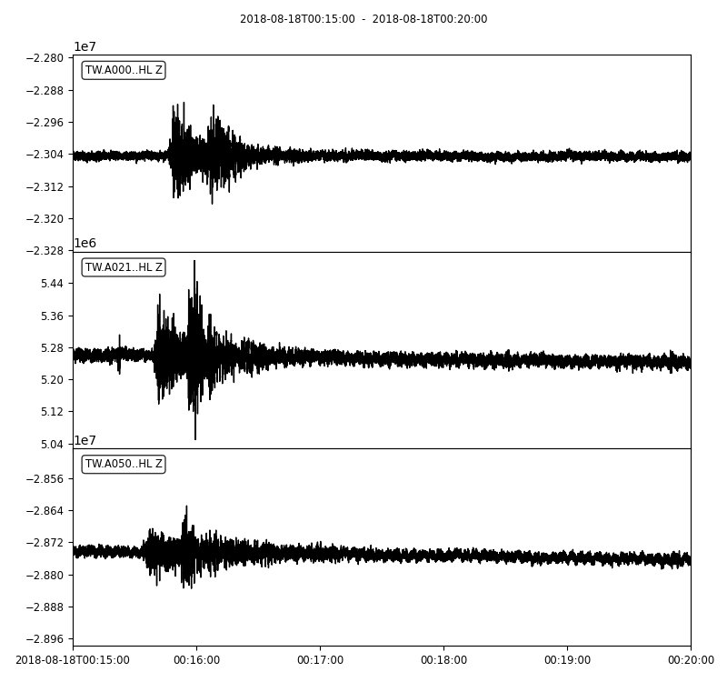
Now, I will create a stream and loop over all the SAC files, create a trace corresponding to each SAC file, add the distance information in the “header” and then add that trace to the stream.
stream = Stream()
for trdata in all_z_data[:3]:
    tr = read(trdata)
    tr[0].stats['distance'] = tr[0].stats.sac.dist*1000
    stream +=tr
stream.plot(outfile='myStream.png',)
The above program for all the traces (350) in our selection, will take a couple of seconds as it has to go through 350 traces of sampling rate upto 200Hz. But still plot size will be huge and hence may throw a ValueError. Hence, we reduce the number of traces to plot in this case. But don’t worry, we will use all the traces for the record section plot.
Detrending and filtering the data
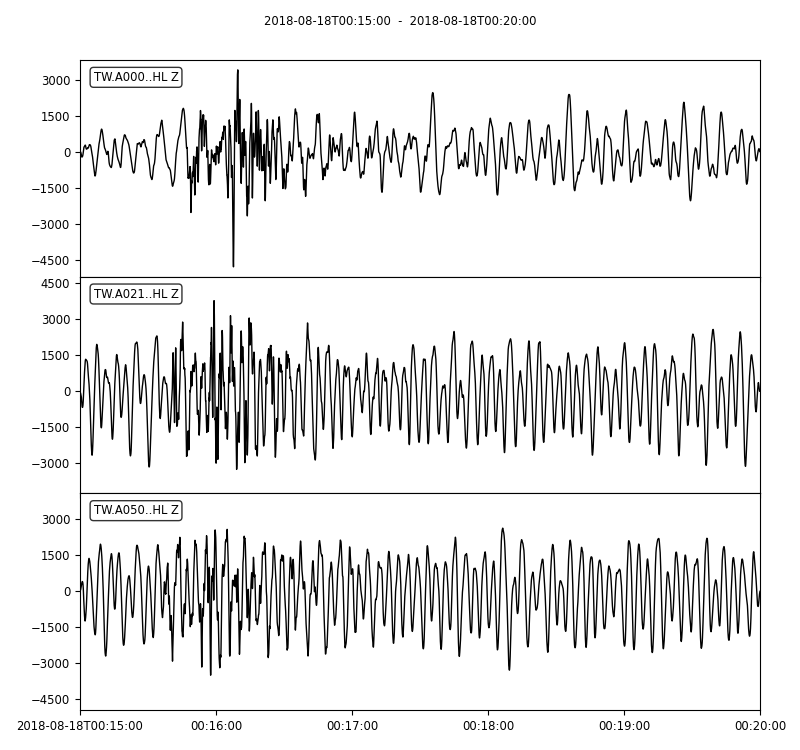
Alternatively, we can detrend and perform bandpass filter to each traces. It is very important to detrend the traces before applying the filter otherwise it may lead to massive artifacts. The Obspy’s filter module provides different filters - bandpass, lowpass, highpass, bandstop and FIR filter.
stream = Stream()
for trdata in all_z_data[:3]:
    tr = read(trdata)
    tr[0].detrend("spline", order=3, dspline=500)
    tr[0].filter("bandpass", freqmin = 1/40, freqmax = 1/5, corners=1, zerophase=True)
    tr[0].stats['distance'] = tr[0].stats.sac.dist*1000
    stream +=tr[0]
stream.plot(outfile='myStream.png',)
Notice that I used the 1/periods instead of the frequencies. The argument corners filter corners (4 by default), and zerophase if “True” apply filter forwards and backwards and hence zero phase shift.
Plot record section
Finally, we are ready to plot the record section. For this, we will use the plot method on the stream and the provide the argument type as section.
from obspy import read, Stream
import glob
all_z_data = glob.glob("*H?Z*-300sec.sac")
stream = Stream()
for trdata in all_z_data:
tr = read(trdata)
tr[0].detrend("spline", order=3, dspline=500)
tr[0].filter("bandpass", freqmin = 1/40, freqmax = 1/5, corners=1, zerophase=True)
tr[0].stats['distance'] = tr[0].stats.sac.dist*1000
stream +=tr[0]
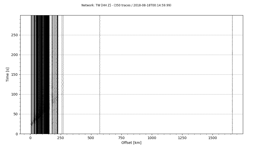
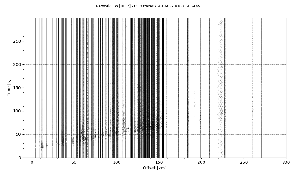
stream.plot(outfile='recordSection1.png',type='section')
The last line will save the stream as a plot of the type section. Notice that, we used all the traces (350 traces read) this time. But the results are difficult to visualize. So, it requires some customization.
The first thing we can do is to get rid of the two traces with distance over 300kms. This may help to properly see the pattern in other traces.
from obspy import read, Stream
import glob
all_z_data = glob.glob("*H?Z*-300sec.sac")
stream = Stream()
for trdata in all_z_data:
tr = read(trdata)
tr[0].detrend("spline", order=3, dspline=500)
tr[0].filter("bandpass", freqmin = 1/40, freqmax = 1/5, corners=1, zerophase=True)
tr[0].stats['distance'] = tr[0].stats.sac.dist*1000
stream +=tr[0]
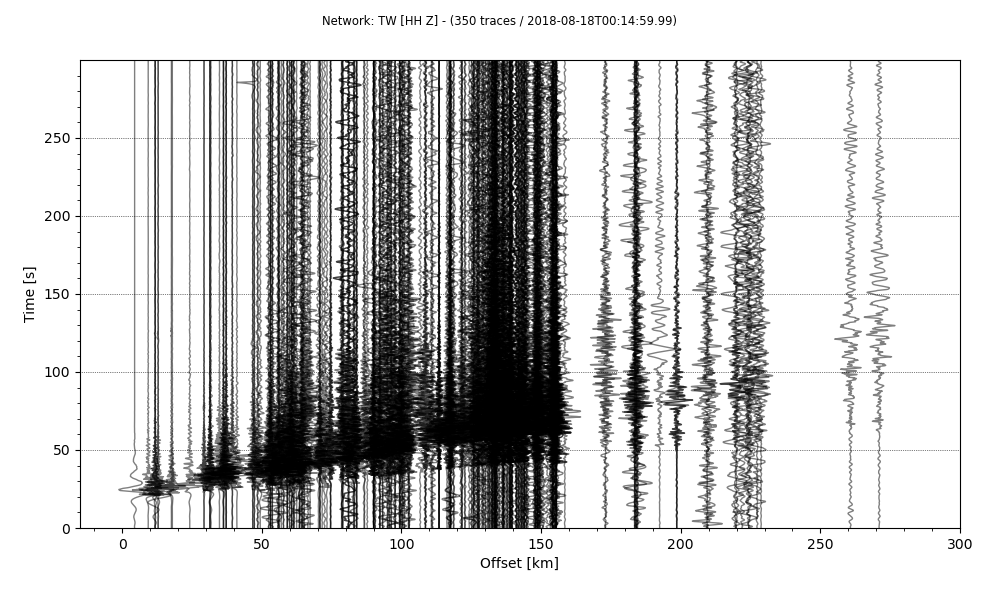
stream.plot(outfile='recordSection1.png',type='section',offset_max=300*1000)
The results are better than before and we started to see some phases but the plot can be more improved. We can scale each traces 10 times to show it better.
from obspy import read, Stream
import glob
all_z_data = glob.glob("*H?Z*-300sec.sac")
stream = Stream()
for trdata in all_z_data:
tr = read(trdata)
tr[0].detrend("spline", order=3, dspline=500)
tr[0].filter("bandpass", freqmin = 1/40, freqmax = 1/5, corners=1, zerophase=True)
tr[0].stats['distance'] = tr[0].stats.sac.dist*1000
stream +=tr[0]
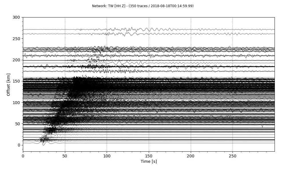
stream.plot(outfile='recordSection1.png',type='section',offset_max=300*1000, scale=10,)
The results this time is much improved. But I prefer time to be on the horizontal axis and the offset on the vertical axis. This can be achieved simply by providing orientation argument.
from obspy import read, Stream
import glob
all_z_data = glob.glob("*H?Z*-300sec.sac")

stream = Stream()
for trdata in all_z_data:
    tr = read(trdata)
    tr[0].detrend("spline", order=3, dspline=500)
    tr[0].filter("bandpass", freqmin = 1/40, freqmax = 1/5, corners=1, zerophase=True)
    tr[0].stats['distance'] = tr[0].stats.sac.dist*1000
    stream +=tr[0]

stream.plot(outfile='recordSection1.png',type='section',offset_max=300*1000, scale=10, orientation='horizontal')
Reducing the linewidth of the plots, makes the figure appear less crowded. The linewidth can be easily reduced.
from obspy import read, Stream
import glob
all_z_data = glob.glob("*H?Z*-300sec.sac")

stream = Stream()
for trdata in all_z_data:
    tr = read(trdata)
    tr[0].detrend("spline", order=3, dspline=500)
    tr[0].filter("bandpass", freqmin = 1/40, freqmax = 1/5, corners=1, zerophase=True)
    tr[0].stats['distance'] = tr[0].stats.sac.dist*1000
    stream +=tr[0]

stream.plot(outfile='recordSection1.png',type='section',offset_max=300*1000, scale=10, orientation='horizontal', linewidth=0.5)
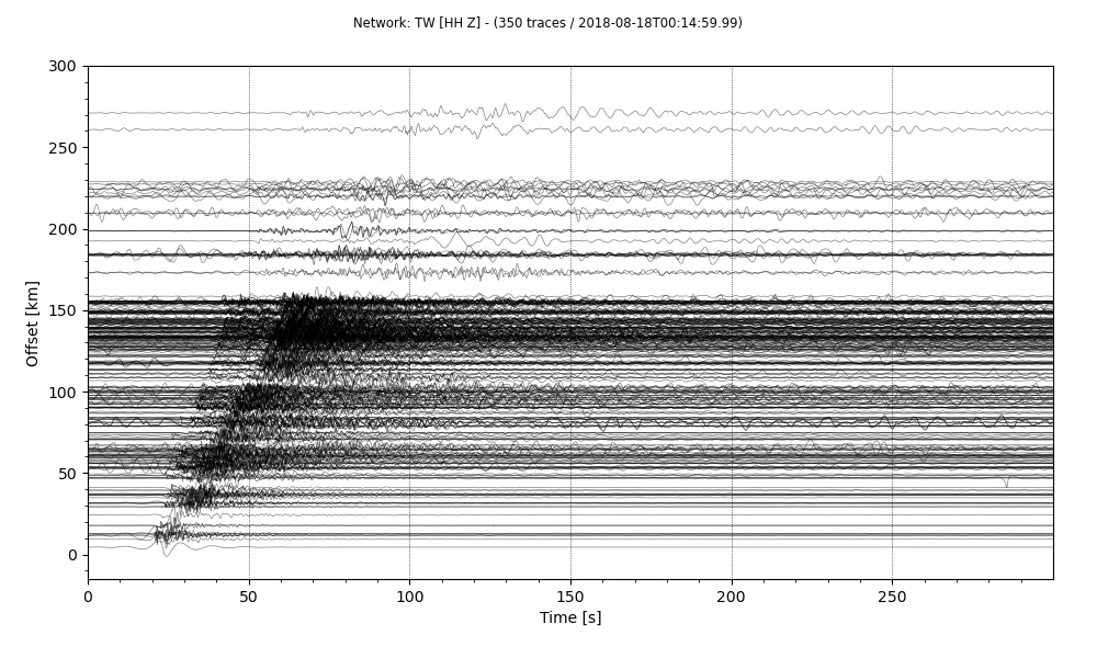
So, we have our final record section. There are a lot more customizations we can do to this plot. Some of them are as easy as changing the arguments to the plot method. You can have a look at the other arguments for the plot in the Obspy’s documentation.
Plot record section for synthetic seismograms
Now, we use the plot the record section for the synthetic seismogram. I use the instaseis database that uses AxiSEM to precompute the green’s functions. I strongly recommend the reader to have a look at the instaseis documentation for details.
## Import libraries
import obspy
import instaseis
import matplotlib.pyplot as plt
import numpy as np
from obspy.core import UTCDateTime
%matplotlib inline
plt.style.use('seaborn')
db = instaseis.open_db('./20s_PREM_ANI_FORCES/') #requires precomputed green functions
## Specify receivers
recvr = instaseis.Receiver(latitude=0., longitude=0., network='SN', station='XYZ')
src = instaseis.Source(
latitude=10.,
longitude=15.,
depth_in_m = 1500.,
m_rr = 4.71e+17,
m_tt = 3.81e+15,
m_pp =-4.74e+17,
m_rt = 3.99e+16,
m_rp =-8.05e+16,
m_tp =-1.23e+17,
origin_time=UTCDateTime(2020, 1, 1, 0, 0)
)
st = db.get_seismograms(
source = src,
receiver = recvr,
components = 'ZRT',
dt = 0.05,
)
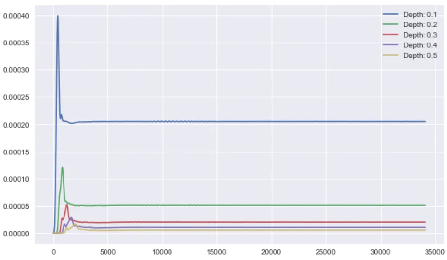
fig, ax = plt.subplots(figsize=(10, 6))
for depth in np.arange(100, 600, 100):
print(depth)
src = instaseis.Source(latitude = 0.0,
longitude=0.,
depth_in_m = depth * 1e3,
m_rr = 4.71e+17,
m_tt = 3.81e+15,
m_pp =-4.74e+17,
m_rt = 3.99e+16,
m_rp =-8.05e+16,
m_tp =-1.23e+17, )
st = db.get_seismograms(
source = src,
receiver = recvr,
components = 'ZRT',
dt = 0.05,)
plt.plot(st[0].data,
label=f"Depth: {depth/1000.}")
plt.legend()
Environment note. plt.style.use('seaborn') was removed in matplotlib 3.8 — use plt.style.use('seaborn-v0_8') (or import seaborn as sns; sns.set_theme()). Everything else here runs on current tooling: the ObsPy read/Stream/stream.plot(type='section', ...) API (including offset_max, scale, orientation, linewidth) is unchanged in ObsPy 1.5, and Instaseis still serves synthetic seismograms from precomputed databases.
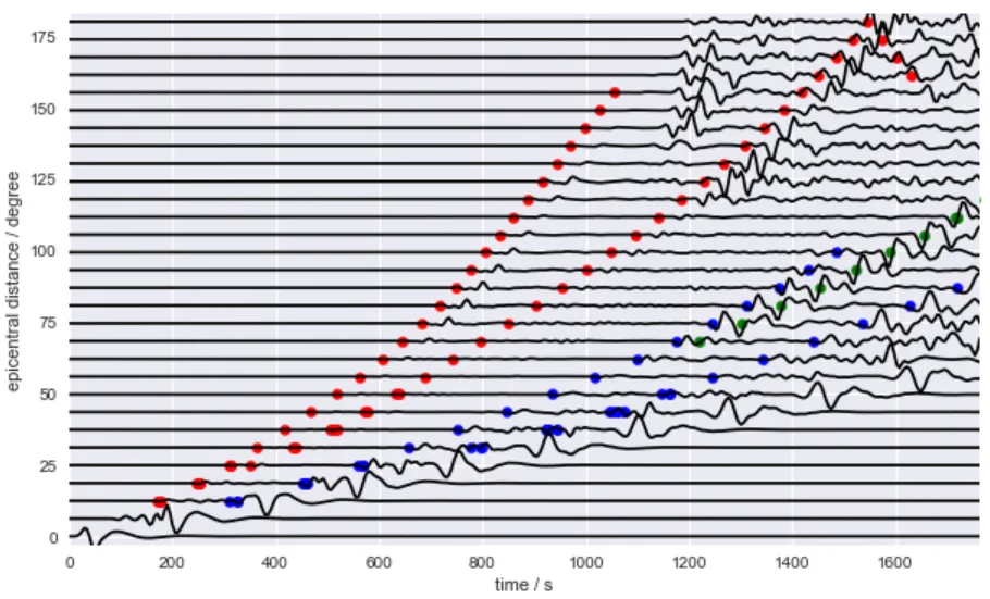
## Slightly modified after the instaseis documentation

from obspy.taup import TauPyModel
from collections import defaultdict

m = TauPyModel(model="ak135")

# some paramters
depth_in_km = 150.
mindist = 0.
maxdist = 180.
numrec = 30
fmin = 0.008
fmax = 0.05
component = "Z"
phases = ["P", "PP", "Pdiff", "S", "SS", "PS"]
colors = ["r", "r", "r", "b", "b", "g"]

# define instaseis source
src = instaseis.Source.from_strike_dip_rake(
    latitude=0., longitude=0.,
    depth_in_m=depth_in_km * 1e3,
    M0=1e+21, strike=32., dip=62., rake=90.)

# storage for traveltimes
distances = defaultdict(list)
ttimes = defaultdict(list)

fig, ax = plt.subplots(figsize=(10, 6))
# loop over distances
for dist in np.linspace(mindist, maxdist, numrec):
    # define receiver
    rec = instaseis.Receiver(latitude=0, longitude=dist)

    # generate seismogram, filter and plot
    tr = db.get_seismograms(source=src, receiver=rec, components=[component])[0]
    tr.filter('highpass', freq=fmin)
    tr.filter('lowpass', freq=fmax)
    tr.normalize()
    plt.plot(tr.times(), tr.data * 5 + dist, color="black")

    # get traveltimes
    arrivals = m.get_travel_times(distance_in_degree=dist,
                                  source_depth_in_km=depth_in_km,
                                  phase_list=phases)
    for arr in arrivals:
        distances[arr.name].append(dist)
        ttimes[arr.name].append(arr.time)

# plot traveltimes
for color, phase in zip(colors, phases):
    plt.scatter(ttimes[phase], distances[phase], s=40, color=color)

plt.xlim(tr.times()[0], tr.times()[-1])
plt.ylim(mindist - 3, maxdist + 3)
plt.xlabel('time / s')
plt.ylabel('epicentral distance / degree')
plt.show()
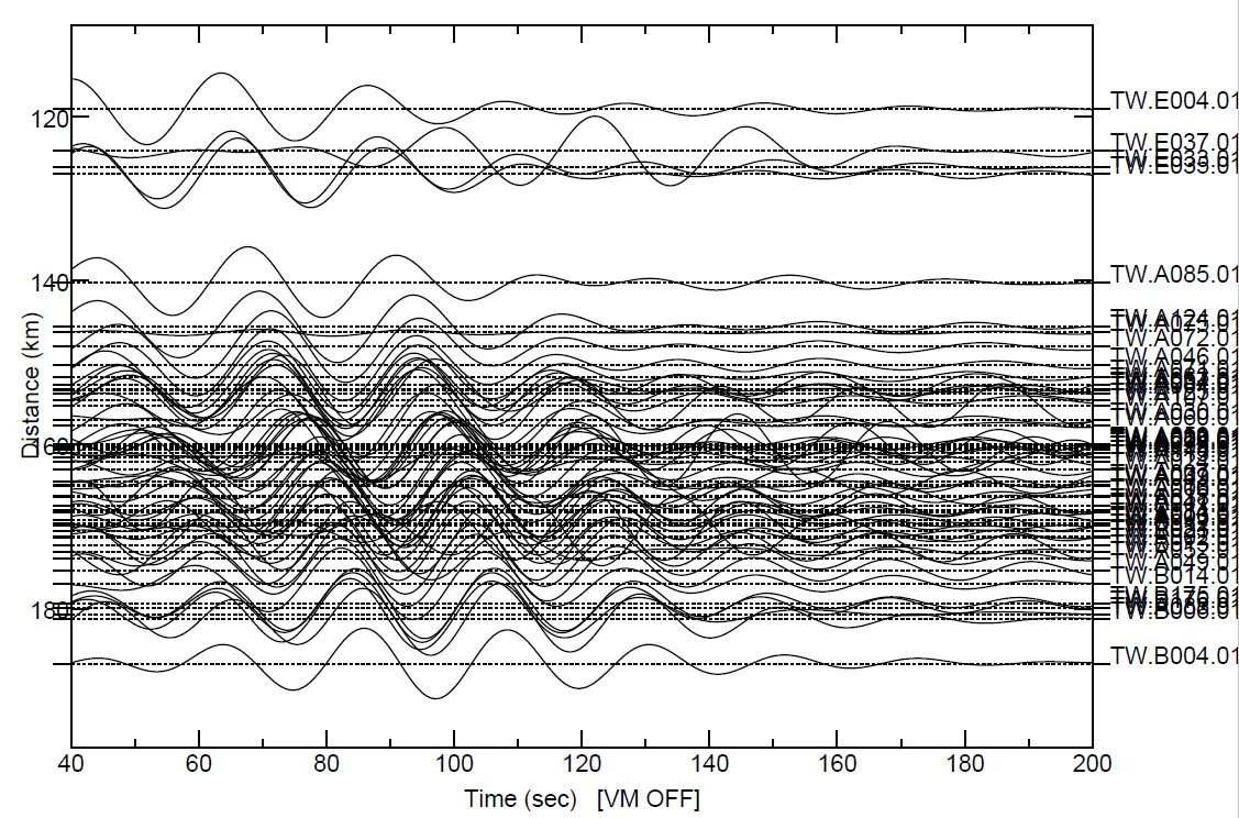
Plotting record section using SAC
Traditionally, seismologists have been using the SAC software to plot the record section. The steps are quite simple and straightforward. But the sac data need to have the epicentral distance in the header. I prepared the sac data using Obspy. But if you have sac data ready then you can skip this step.
Prepare SAC data
from obspy import read
import glob, os
from obspy.io.sac.sactrace import SACTrace
import pandas as pd

## Some header info is stored in the text file
df_info = pd.read_csv('data_info_20181023_160404-CWBTS.txt')
print(df_info.head())
The format of the header info is following:
  network station channel     stla      stlo  stel     evla      evlo  evdp                    starttime                      endtime  samplingRate    dist     baz
0      TW    A002     HLZ  25.1258  121.4669  10.0  23.9932  122.6308  30.1  2018-10-23T16:03:34.002501Z  2018-10-23T16:10:44.002501Z         100.0  172.17  136.53
1      TW    A003     HLZ  25.0860  121.4571  11.0  23.9932  122.6308  30.1  2018-10-23T16:03:34.002501Z  2018-10-23T16:10:44.002501Z         100.0  169.69  135.26
2      TW    A006     HLZ  25.0940  121.5152   8.0  23.9932  122.6308  30.1  2018-10-23T16:03:34.000000Z  2018-10-23T16:10:44.000000Z         100.0  166.26  136.94
3      TW    A007     HLZ  25.0735  121.5168   9.0  23.9932  122.6308  30.1  2018-10-23T16:03:34.000000Z  2018-10-23T16:10:44.000000Z         100.0  164.50  136.44
4      TW    A009     HLZ  25.0794  121.5811  12.0  23.9932  122.6308  30.1  2018-10-23T16:03:34.000000Z  2018-10-23T16:10:44.000000Z         100.0  160.59  138.30
## the mseed file is located in the StR and StZ directories
stR = read("StR/region1_stream_HLR_20181023_160404-CWBTS.mseed")
stZ = read("StZ/region1_stream_HLZ_20181023_160404-CWBTS.mseed")

for tr in stR:
    sacf = f"stR/{tr.id}.SAC"
    tr.write(sacf, format='SAC')
    sac1 = SACTrace.read(sacf)
    df_tr = df_info[(df_info["network"] == tr.stats.network) & (df_info["station"] == tr.stats.station)]
    sac1.evla=evla
    sac1.evlo=evlo
    sac1.evdp=evdp
    sac1.stla = df_tr["stla"].values[0]
    sac1.stlo = df_tr["stlo"].values[0]
    sac1.stel = df_tr["stel"].values[0]
    sac1.dist = df_tr["dist"].values[0]
    sac1.baz = df_tr["baz"].values[0]
    sac1.write(sacf, headonly=True)

for tr in stZ:
    sacf = f"stZ/{tr.id}.SAC"
    tr.write(sacf, format='SAC')
    sac1 = SACTrace.read(sacf)
    df_tr = df_info[(df_info["network"] == tr.stats.network) & (df_info["station"] == tr.stats.station)]
    sac1.evla=evla
    sac1.evlo=evlo
    sac1.evdp=evdp
    sac1.stla = df_tr["stla"].values[0]
    sac1.stlo = df_tr["stlo"].values[0]
    sac1.stel = df_tr["stel"].values[0]
    sac1.dist = df_tr["dist"].values[0]
    sac1.baz = df_tr["baz"].values[0]
    sac1.write(sacf, headonly=True)
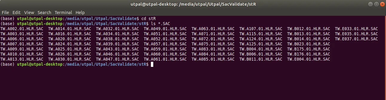
This will save the sac file with prefix “SAC” in the respective stZ and stR directories.
Now, we can head to the SAC software and navigate to the directory containing the SAC data.
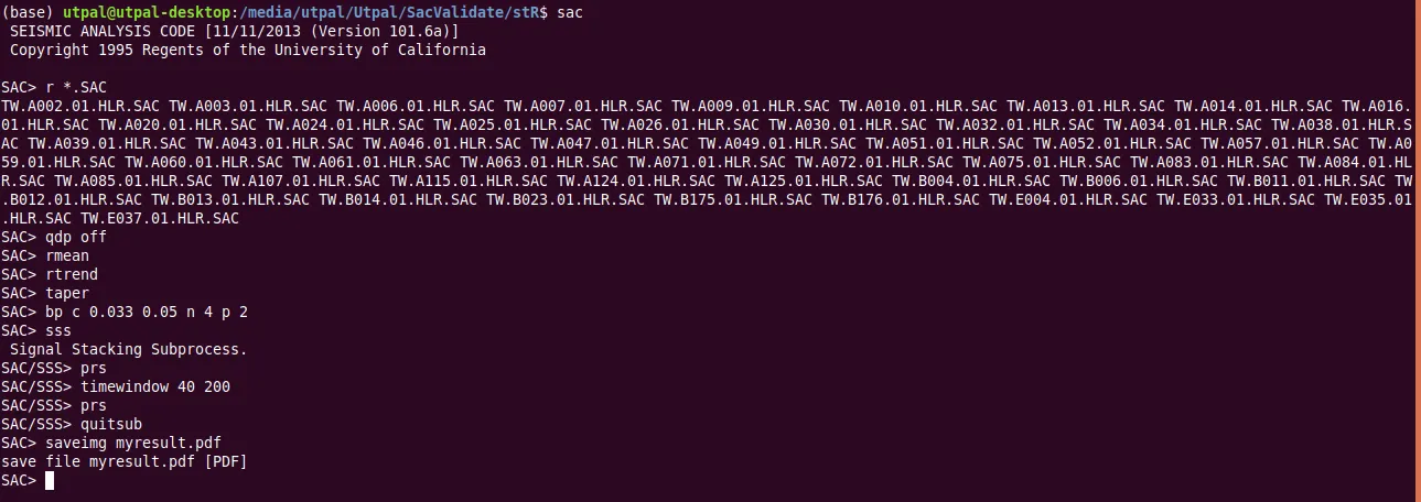
SAC Commands are
r *.SAC # read all sac files in the directory
qdp off
rmean
rtrend
taper
bp c 0.033 0.05 n 4 p 2 #bandpass filter between 20-30s with filter corners with order 4 and filter once forwards and once backwards
sss #start signal stacking subprocess
timewindow 40 200 #set time window
prs #plotrecordsection
quitsub #quit the subprocess
saveimg myresult.pdf #save the plot as pdf
Quick check: Before stream.plot(type='section') will work, what must each trace carry?
- Its sampling rate in
tr.stats.sampling_rate - Its epicentral distance in
tr.stats.distance(in metres) - A
matplotlibcolormap in the header - The earthquake magnitude in
tr.stats.mag
Recap
- A record section plots each seismogram at a height set by its epicentral distance, so the first arrivals form a moveout whose slope is the apparent velocity.
- The one prerequisite is
tr.stats.distancein metres — here it is set from the SAC header viatr.stats.sac.dist * 1000. - Detrend before filtering (
tr.detrend(...)thentr.filter("bandpass", ...)), otherwise the filter introduces artifacts;zerophase=Truefilters forwards and backwards for no phase shift. stream.plot(type='section', ...)accepts handy tweaks —offset_max,scale,orientation='horizontal', andlinewidth— all unchanged in current ObsPy.- The same idea works for synthetics (Instaseis + TauPy travel times) and in the classic SAC software (
sss→prs).
Where to go next
- Automatically plotting a seismic section in Python — a scripted take on the same plot.
- Getting started with ObsPy for seismologists — the fundamentals of
read,Stream, andTrace. - Concatenating daily seismic traces and plotting a spectrogram — more ObsPy waveform handling.
- Automatically enquire seismic data availability with ObsPy — where to fetch the waveforms in the first place.
References
- van Driel, M., Krischer, L., Stähler, S. C., Hosseini, K., and Nissen-Meyer, T. (2015). Instaseis: instant global seismograms based on a broadband waveform database. Solid Earth, 6, 701-717.
Disclaimer of liability
The information provided by the Earth Inversion is made available for educational purposes only.
Whilst we endeavor to keep the information up-to-date and correct. Earth Inversion makes no representations or warranties of any kind, express or implied about the completeness, accuracy, reliability, suitability or availability with respect to the website or the information, products, services or related graphics content on the website for any purpose.
UNDER NO CIRCUMSTANCE SHALL WE HAVE ANY LIABILITY TO YOU FOR ANY LOSS OR DAMAGE OF ANY KIND INCURRED AS A RESULT OF THE USE OF THE SITE OR RELIANCE ON ANY INFORMATION PROVIDED ON THE SITE. ANY RELIANCE YOU PLACED ON SUCH MATERIAL IS THEREFORE STRICTLY AT YOUR OWN RISK.
Leave a comment