Simple wave modeling and Hilbert Transform in Matlab (codes included)

Utpal Kumar 4 minute read GEOPHYSICS October 23, 2020

Introduction

We can use waves to model almost everything in the world from the thing we can see or touch to the things which we can’t.

Here, we try to model the waves itself.

Key idea — a moving wave, its spectrum, and its envelope. A travelling wave is $y = a\sin(kx - \omega t)$: fix the time and step it forward and the pattern slides along $x$. The Fourier transform (fft) tells you which frequencies build a signal. The Hilbert transform (hilbert) does something different — it builds the analytic signal $x + i\,\mathcal{H}(x)$, whose magnitude is the smooth envelope that traces the signal’s instantaneous amplitude. That envelope is the workhorse here: it finds edges in a signal and tracks how a wave group moves when different frequencies travel at different speeds (dispersion).

The Hilbert transform turns a signal into its analytic form; the magnitude of that is the envelope tracing the peaks.

Moving Waves

clear; close all; clc
a=1;    %amplitude
f=5;    %frequency
T=1/f;  %time period
w=2*pi*f;   %angular frequency
lb=2*T; %wavelength
k=2*pi/lb; %wavenumber
x=0:pi/200:10*pi;
t=0:0.01:2; %time
figure(1)
for i=1:length(t)
    y=a*sin(k*x-w*t(i));    %waveform
    plot(x,y)
    pause(0.1)
end

Snapshot of a single travelling sine wave

Fourier Transform to analyse the amplitude spectrum

clear; close all; clc
fs=1000;    %sampling frequency
t=0:1/fs:1.5-1/fs;%time
f1=10;  %frequency1
f2=20;  %frequency2
f3=30;  %frequency3
%x=5*sin(2*pi*10*t+3);
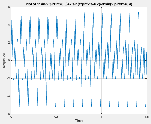
x=1*sin(2*pi*f1*t+0.3)+2*sin(2*pi*f2*t+0.2)+3*sin(2*pi*f3*t+0.4);
plot(t,x)
figure(1)
grid on
xlabel('Time')
ylabel('Amplitude')
title('Plot of 2*sin(2*pi*f1*t+0.3)-3*sin(2*pi*f2*t+0.2)+5*cos(2*pi*f3*t+0.4)')
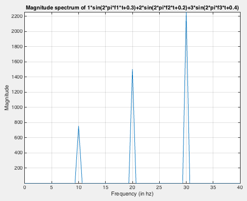
X=fft(x);
fre=fs/length(t);
fre_hz=(0:length(t)/2-1)*fre;
X_mag=abs(X);   %X is complex
figure(2)
plot(fre_hz,X_mag(1:length(t)/2))
grid on
axis([0 40 -inf inf])
xlabel('Frequency (in hz)')
ylabel('Magnitude')
title('Magnitude spectrum of 5*sin(2*pi*10*t+3)')

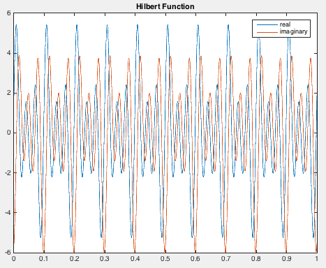
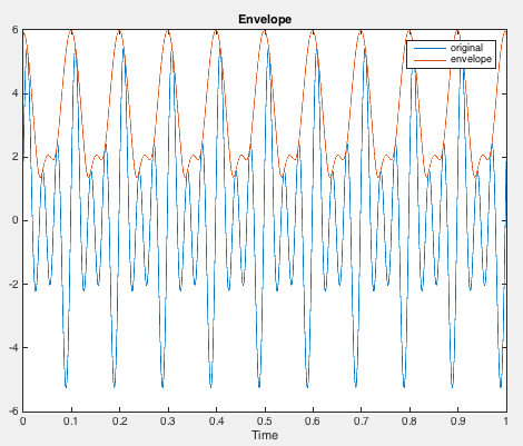
A three-frequency signal in the time domain The FFT magnitude spectrum showing peaks at 10, 20 and 30 Hz

Hilbert Transform and get the envelope of the waveform

clear; close all; clc
fs = 1e4;   %sampling frequency
t = 0:1/fs:1;   %time
f1=10;
f2=20;
f3=30;
x=1*sin(2*pi*f1*t+0.3)+2*sin(2*pi*f2*t+0.2)+3*sin(2*pi*f3*t+0.4);
%x=5*sin(2*pi*10*t+3);
y = hilbert(x);
figure(1)
plot(t,real(y),t,imag(y))
% %xlim([0.01 0.03])
legend('real','imaginary')
title('Hilbert Function')
figure(2)
env=abs(y);
plot(t,x)
xlabel('Time')
title('Envelope')
hold on
plot(t,env)
legend('original','envelope')

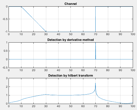
Real and imaginary parts of the Hilbert analytic signal A signal with its Hilbert-transform envelope overlaid

Application of Hilbert Transform: Edge Detection and comparison with the classical derivative method

clear; close all; clc
x = 0:0.1:100;
y = channel(x,[10 30 70]);  %channel function to define a trapezoidal channel
plot(x,y)
figure(1)
subplot(311)
plot(x,y)
grid on
title('Channel')

subplot(312)
deriv =diff(y); %dervative of the channel
plot(x(2:end),deriv)
title('Detection by derivative method')
grid on

subplot(313)
hil = hilbert(y);   %hilbert transform of the channel
env=abs(hil);
plot(x,env)
grid on
title('Detection by hilbert transform')

Channel Function

function y = channel(x, params)

a = params(1); b = params(2); c = params(3);
for index=1:length(x)
    if x(index)<=a
        y(index)=0;
    elseif (x(index) >= a) && (x(index) <= b)
        y(index)=(x(index)-a)/(a-b);
    elseif (x(index) >= b) && (x(index) < c)
        y(index)=-1;
    elseif (x(index) >= c)
        y(index)=0;
    end
end

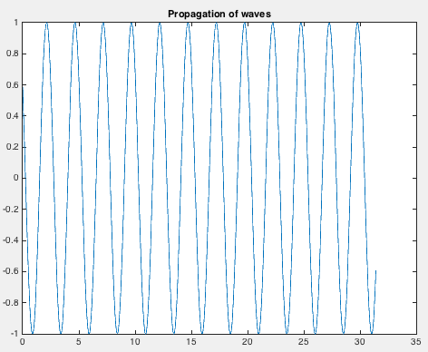
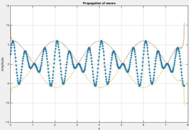
Edge detection: channel signal, derivative method, and Hilbert-transform method

Complex Moving Waves

In nature, usually we encounter waves as an ensemble of many frequencies.

Here, let us try to add more frequencies in the previous scenario. We plot a wave containing three frequencies.

clear; close all; clc
fs=1000;    %sampling frequency
t=0:1/fs:0.5-1/fs;%time
f=[1 2 3];  %frequency1
a=[1 2 3];  %amplitude
c=2; %wave speed
T=1./f;  %time period
w=2*pi*f;   %angular frequency
lb=c*T; %wavelength
k=(2*pi)./lb; %wavenumber
x=0:pi/200:(2.5*pi)-pi/200;
figure('Position',[440 378 800 500])
for i=1:length(t)/2
%     y=a*sin(k*x-w*t(i));    %waveform
    y=a(1)*sin((k(1)*x)-(w(1)*t(i))+0.3)+a(2)*sin((k(2)*x)-(w(2)*t(i))+0.4)+a(3)*sin((k(3)*x)-(w(3)*t(i))+0.5);
    plot(x,y,'--*')
    title('Propagation of waves')
    xlabel('x')
    ylabel('Amplitude')
    grid on
    pause(0.05)
end

We have modelled the wave in which each frequency is travelling with the same velocity. We can add some complexity where every frequency in our wave is travelling with different speed. This is popularly known as dispersion.

Let us model our waves such that the wave speed for 1,2 and 3 Hz is 0.5,1 and 2 km/s.

In this case, we can notice that the waves are travelling in groups and its shape keep changing. We can use the concept of hilbert transform to model the propagation of the group.

Dispersive wave packet whose shape changes as it propagates

Quick check: You have a modulated signal and want the smooth curve that traces its instantaneous amplitude (its envelope). Which MATLAB function gives you that?

fft(x) — the Fourier transform
abs(hilbert(x)) — the magnitude of the analytic signal
diff(x) — the numerical derivative
sin(x) — a sine wave

Recap

A travelling wave is $y = a\sin(kx - \omega t)$; animating over time (the for loop with pause) makes the pattern move along $x$.
fft gives the amplitude spectrum — the frequencies that make up a signal (here, clean peaks at 10, 20, 30 Hz).
hilbert builds the analytic signal; abs(hilbert(x)) is the envelope, the signal’s instantaneous amplitude.
That envelope has two uses shown here: edge detection (it flags where a channel signal turns on/off, cleaner than the noisy derivative) and tracking a dispersive wave group whose shape changes as each frequency travels at a different speed.
All of this uses stock MATLAB (sin, fft, hilbert, diff, plot) — the hilbert function lives in the Signal Processing Toolbox.

Where to go next

Signal denoising using the Fast Fourier Transform — go further with the spectrum you compute here.
Time-frequency analysis in MATLAB — see how frequencies evolve in time, not just overall.
Time-series analysis: filtering and smoothing data — clean up a signal before transforming it.

Disclaimer of liability

The information provided by the Earth Inversion is made available for educational purposes only.

Whilst we endeavor to keep the information up-to-date and correct. Earth Inversion makes no representations or warranties of any kind, express or implied about the completeness, accuracy, reliability, suitability or availability with respect to the website or the information, products, services or related graphics content on the website for any purpose.

UNDER NO CIRCUMSTANCE SHALL WE HAVE ANY LIABILITY TO YOU FOR ANY LOSS OR DAMAGE OF ANY KIND INCURRED AS A RESULT OF THE USE OF THE SITE OR RELIANCE ON ANY INFORMATION PROVIDED ON THE SITE. ANY RELIANCE YOU PLACED ON SUCH MATERIAL IS THEREFORE STRICTLY AT YOUR OWN RISK.