Numerical tests for seismic resolution (codes included)
Introduction
Seismic resolution and fidelity are the two important measures of the quality of the seismic record and the seismic images. Seismic resolution quantifies the level of precision, such as the finest size of the subsurface objects detectable by the seismic data whereas the seismic fidelity quantifies the truthfulness such as the genuineness of the data or the level to which the imaged target position matches its true subsurface position.
Let us try to understand this by making a synthetic data and doing the analysis over it.
Seismic Resolution Analysis: 1
To do the analysis, let us consider a Ricker’s wavelet.
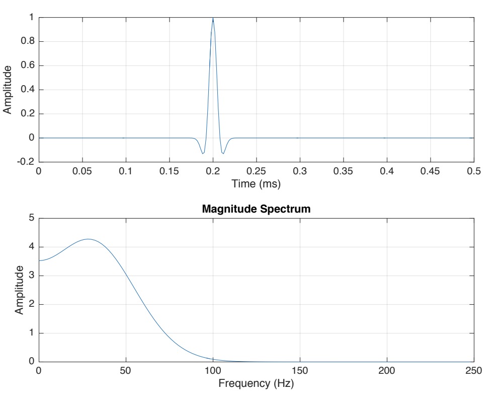
Let us create a zero phase Ricker’s wavelet with 40hz, 250 points and sampling rate of 2 ms. We also plot the amplitude spectrum of it.
Now, let us plot Ricker’s wavelet for 10hz, other parameters being same.
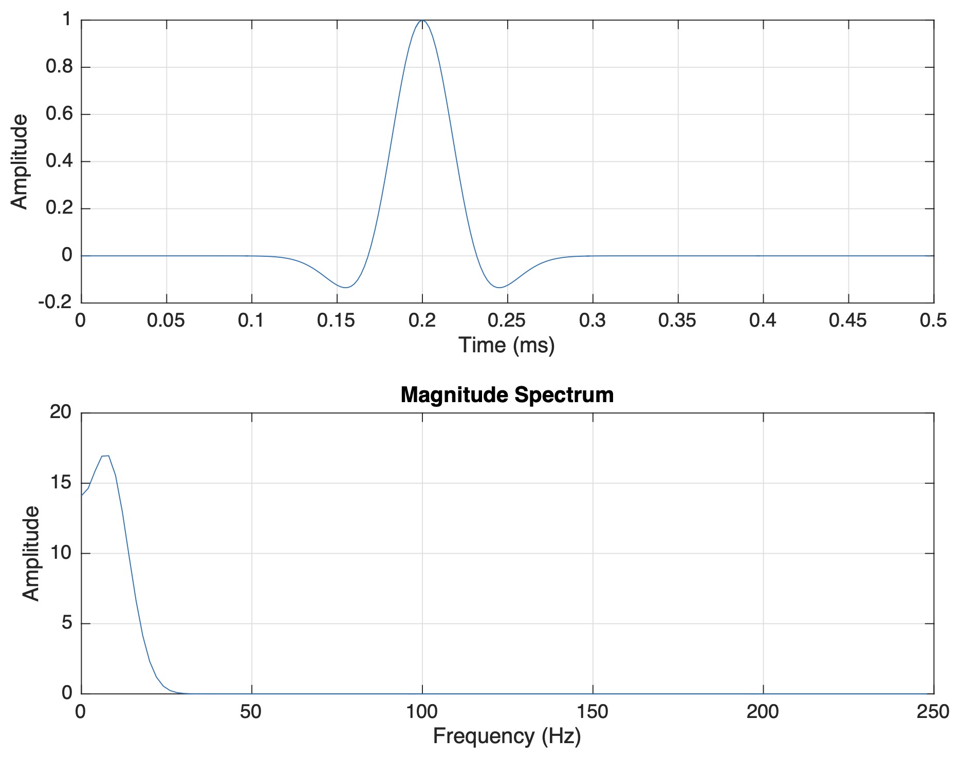
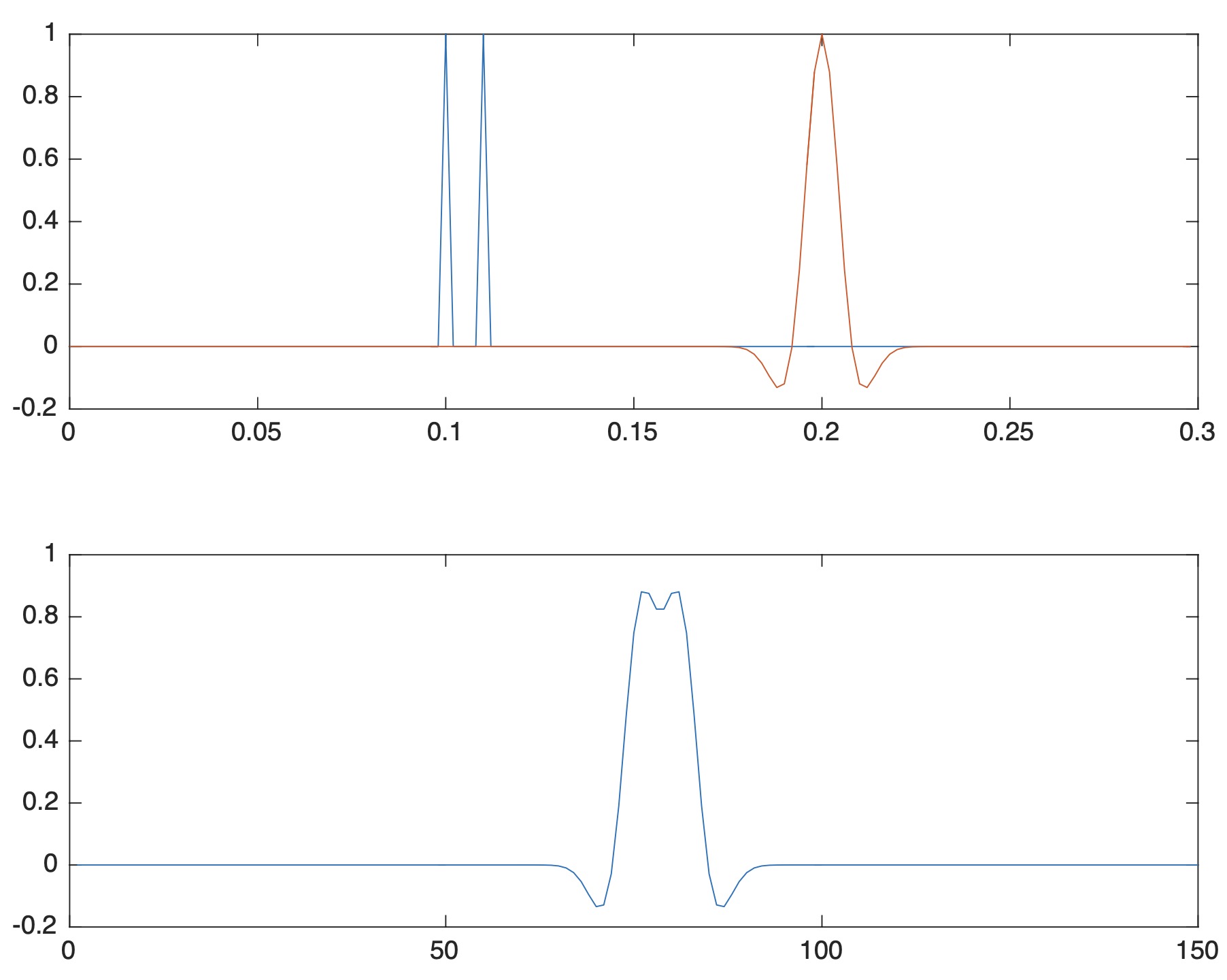
Here, we can clearly observe that the bandwidth of the spectra decreases dramatically and hence we lose the temporal resolution. So, larger the resolution in time domain, lesser the resolution in frequency domain and vice-versa. Now, let us try to use the wavelet analysis to resolve a pair of spiky reflectors. The reflectors are observed to the subsurface interfaces. If the two reflectors are closer then that means the two interfaces are close. If we could resolve the two reflectors, then we can resolve the depth of the bed interfaces. Let us consider a source with Ricker’s wavelet and the two reflectors. If the two reflectors are far enough then it can be easily resolved.
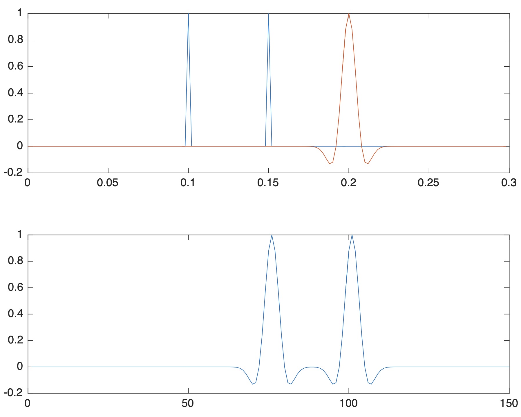
But when the two reflectors are very close then it is difficult to resolve them.
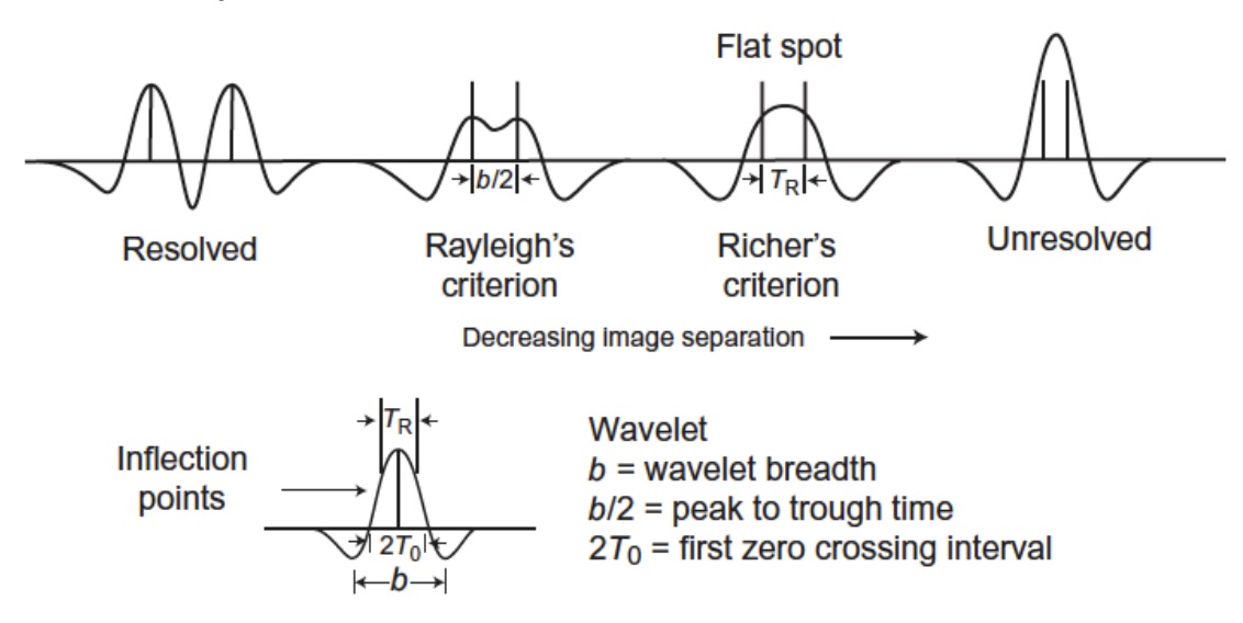
Ricker’s resolution limit is the separation interval between inflection points of the seismic wavelet, i.e., TR in this case. The resolution limit is the width of the wavelet between two inflection points. If we take the wavelet with higher frequency, then the distance between the two inflection points could be reduced. So, lets consider a wavelet with frequency of 80hz (double of the previous case).
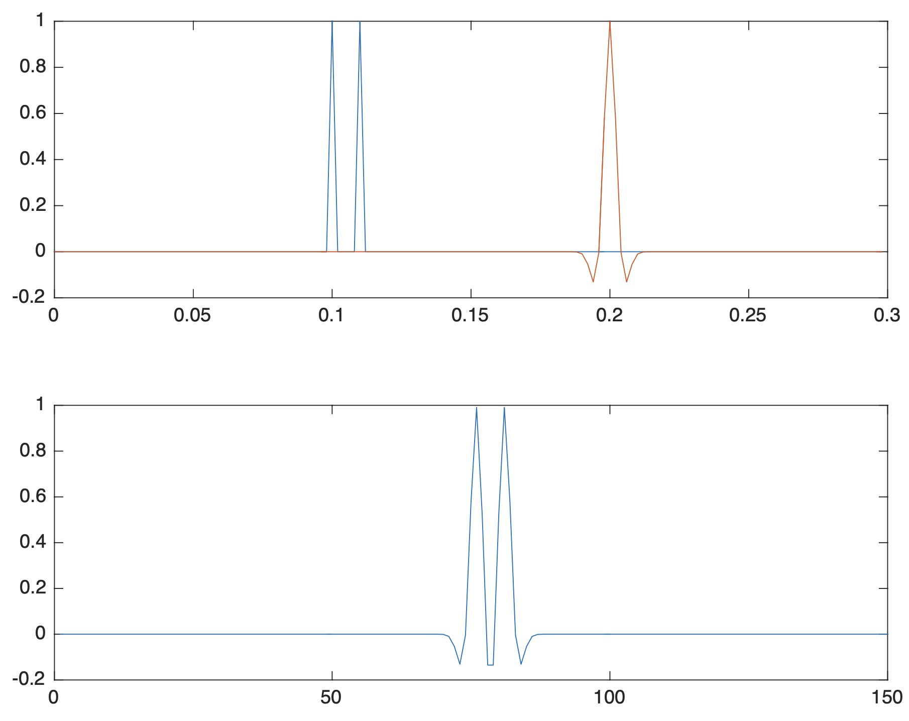
In this case, the two reflectors have been resolved.
\[\begin{aligned} T_R = \frac{\sqrt{6}}{2\pi f_{dom}} \end{aligned}\]The above equation was proposed by Chung and Lawton (1995) for tuning thickness estimation. Through this equation, Ricker wavelet with the dominant frequency of 40hz will have a tuning thickness of 9ms. It means that this 9ms is the tuning separation between two consecutive events in time domain, below this, the event response interference start to dominate and events become visually inseparable.
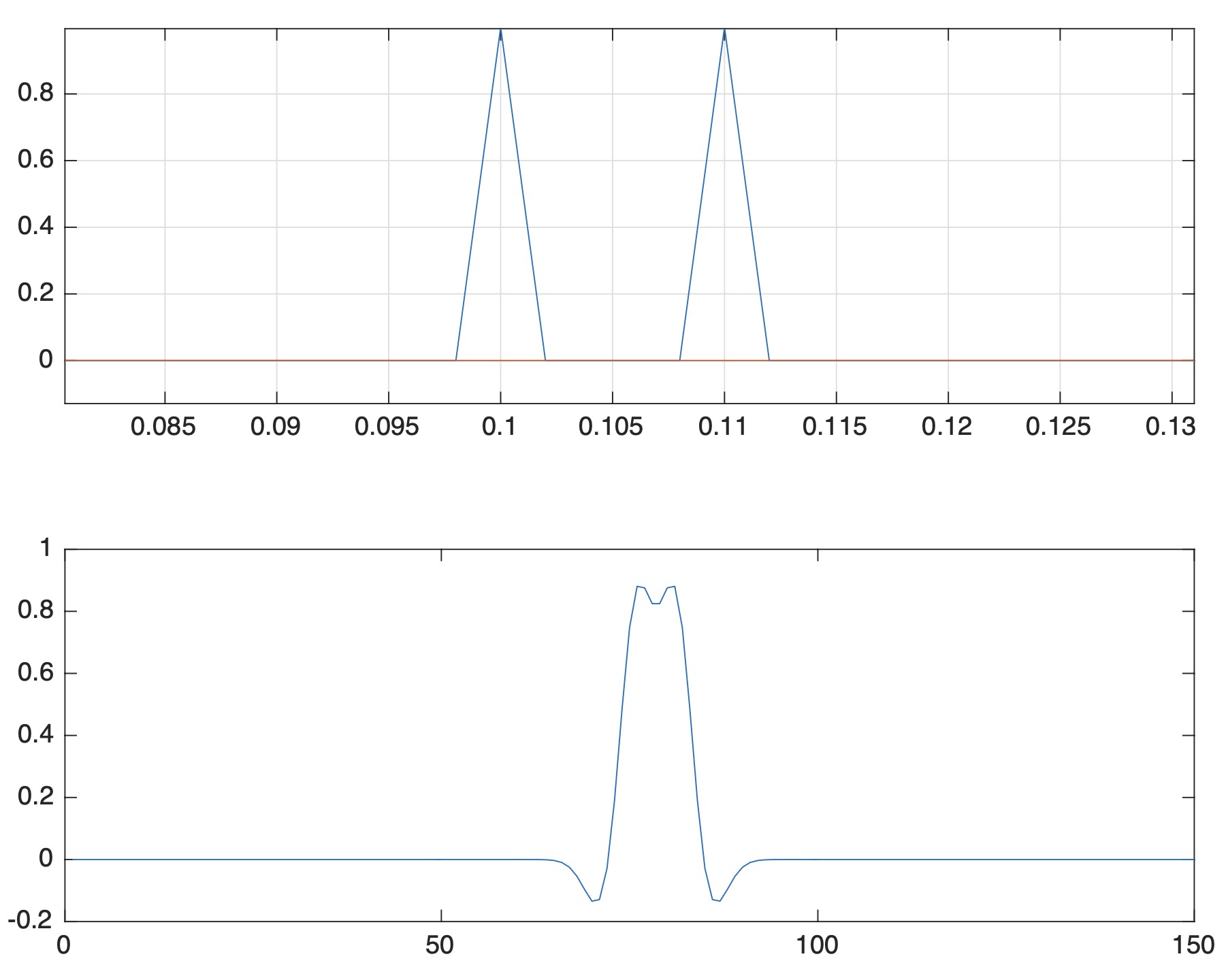
In the above figure for Ricker wavelet of 40hz, the time difference between the two events is 10ms and the events is almost visually inseparable.
MATLAB Codes
clear; close all; clc
dt=0.002;
t=0:dt:0.3-dt;

for i=1:length(t)
  if t(i)==0.1 || t(i)==0.11
    x(i)=1;
  else
    x(i)=0;
  end
end
[rw,t] = ricker(80,length(x),dt,0.2);

figure(1)
subplot(211)
plot(t,x,t,rw)
grid on
x_rw_conv=conv(x,rw,'same');

subplot(212)
plot(x_rw_conv)
Estimation of the Width of the Fresnel’s Zone
The Fresnel’s resolution quantifies the resolvability of seismic wave perpendicular to the direction of wave propagation. Fresnel’s resolution is defined as the width of the first Fresnel’s zone due to interference of the spherical waves from the source and from the receiver.
Seismic Resolution Analysis: 2
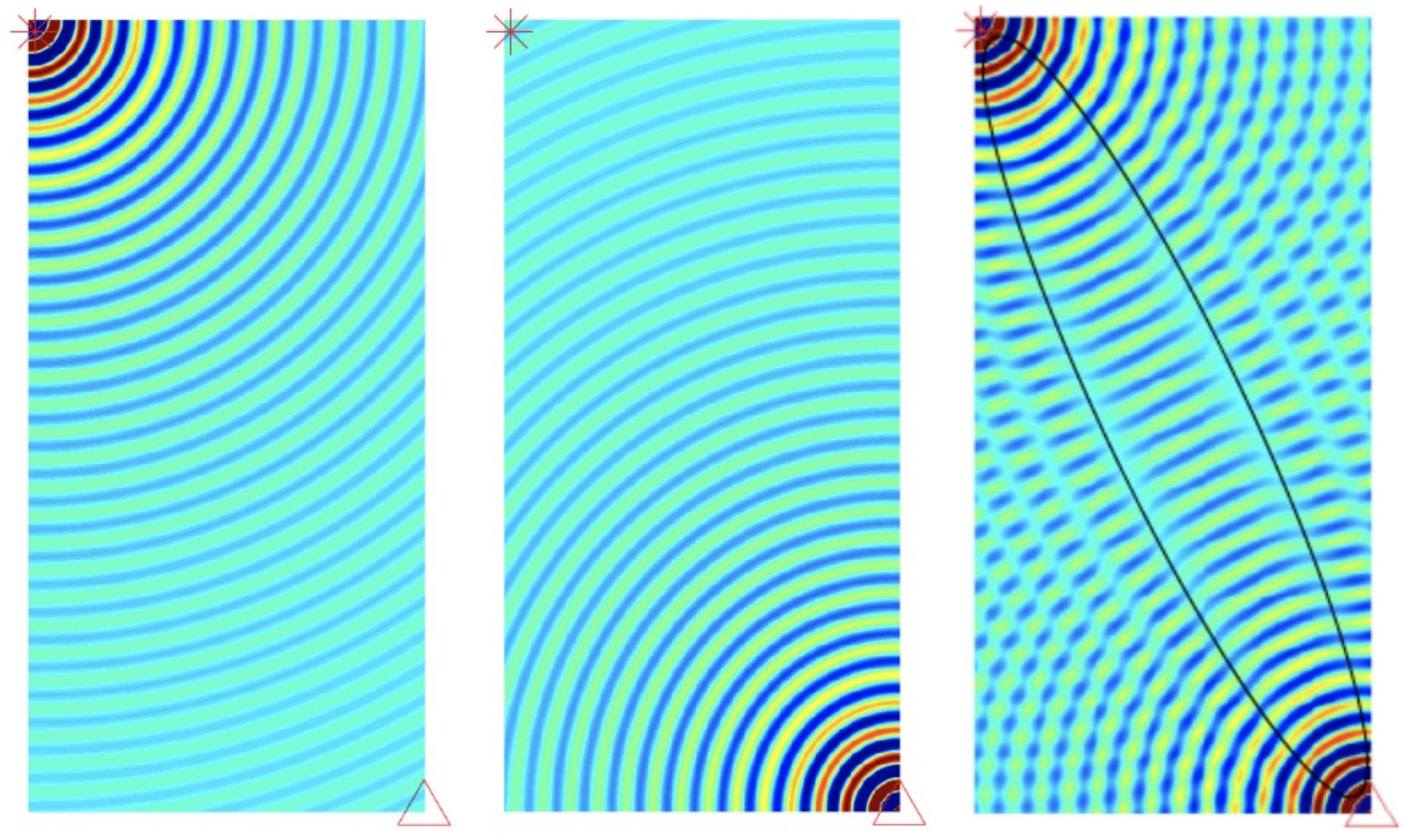
For the above simulation, we have considered a monochromatic spherical wave of wavenumber 100 m-1 and frequency 1 hz at a distance of 2012 metres.
Equation for the wave propagation is
\[\begin{aligned} u(r,t) = \frac{1}{r}e^{i(\omega t - kr)} \end{aligned}\]The width of the first fresnel’s zone is
\[\begin{aligned} W = \sqrt{2d\lambda + \lambda^2/4} \end{aligned}\]So, for our case, \(𝑊 = \sqrt{2 \times 2012 \times 0.01 + 0.01^2/4} = 6.3435\) meters
MATLAB Codes
clear; close all; clc
% an illustration of a spherical wave
filename = 'wave_propagation.gif';
h=figure;
set(h,'color','w','Position',[440 122 350 1000])
Lx = 0.9;
Ly=1.8;
factor = 5;
shift = 5;

Mx = Lx/2;
Wy = Ly/2;

M=400;
N = floor(M*Ly/Lx);

[X, Y]=meshgrid(linspace(0, Lx, M), linspace(-Ly, 0, N));
[Xr, Yr]=meshgrid(linspace(-Lx, 0, M), linspace(0, Ly, N));

wavenumber = 100;

T = 1;
nt = 20;
Time = linspace(0, T, nt);

for repeat = 1:1
  % go over one time period of the field
  for iter = 1:(nt-1) % nt is same as 1 due to peridicity
    t = Time(iter);
    % spherical wave
    Z = exp(sqrt(-1)*wavenumber*sqrt(X.^2+Y.^2))*exp(-sqrt(- 1)*2*pi*t)./sqrt(X.^2+Y.^2);
    Zr = exp(sqrt(-1)*wavenumber*sqrt(Xr.^2+Yr.^2))*exp(-sqrt(- 1)*2*pi*t)./sqrt(Xr.^2+Yr.^2);
  end

  % plot the real part of the field Z
  figure(1);
  clf;
  hold on;
  axis equal;
  axis off;
  image(factor*(real(Z+Zr+shift))); % add shift to Z for graphing purposes
  plot(7,788,'*r','MarkerSize',20)

  plot(400,3,'^r','MarkerSize',20)
  title('Wave propagation and Fresnels Zone')

  colormap jet; shading interp;
  drawnow
  frame = getframe(1);
  im = frame2im(frame);
  [A,map] = rgb2ind(im,256);
  if iter == 1;
    imwrite(A,map,filename,'gif','LoopCount',Inf,'DelayTime',1);
  else
    imwrite(A,map,filename,'gif','WriteMode','append','DelayTime',1);
  end
  file = sprintf('wave_frame%d.png', 1000+iter);
  disp(file); %show the frame number we are at
  print(file,'-dpng')
  pause(0.1);
end
Fidelity
To investigate the fidelity of our data, let us consider the technique of resampling. For our case we consider the method of “bootstrapping”. Bootstrapping basically relies on random sampling with replacement. The other popular method for resampling is “jackknifing” which predates “bootstrapping”. The jackknife estimator of a parameter is found by systematically leaving out each observation from a dataset and calculating the estimate and then finding the average of these calculations.
The principle behind “bootstrapping” is that a dataset is taken, the total dataset is divided into two by randomly sampling with replacement. The newly sampled data are now used to invert for the model using some kernel function. If the two models correlate high enough then we can say that the prominent features in the model come from consistent signals in the data.
We don’t have the data set to make the velocity model. So instead, we can take random Gaussian distribution data and play with it.
Let’s pose the null hypothesis that the two sets of data come from the same probability distribution (not necessarily Gaussian). Under the null hypothesis, the two sets of data are interchangeable, so if we aggregate the data points and randomly divide the data points into two sets, then the results should be comparable to the results obtained with the original data. So, the strategy is to generate random datasets, with replacement (bootstrapping), compute difference in means (or difference in medians or any other reliable statistic), and then compare the resulting values to the statistic computed from the original data.
Seismic Resolution Analysis: 3
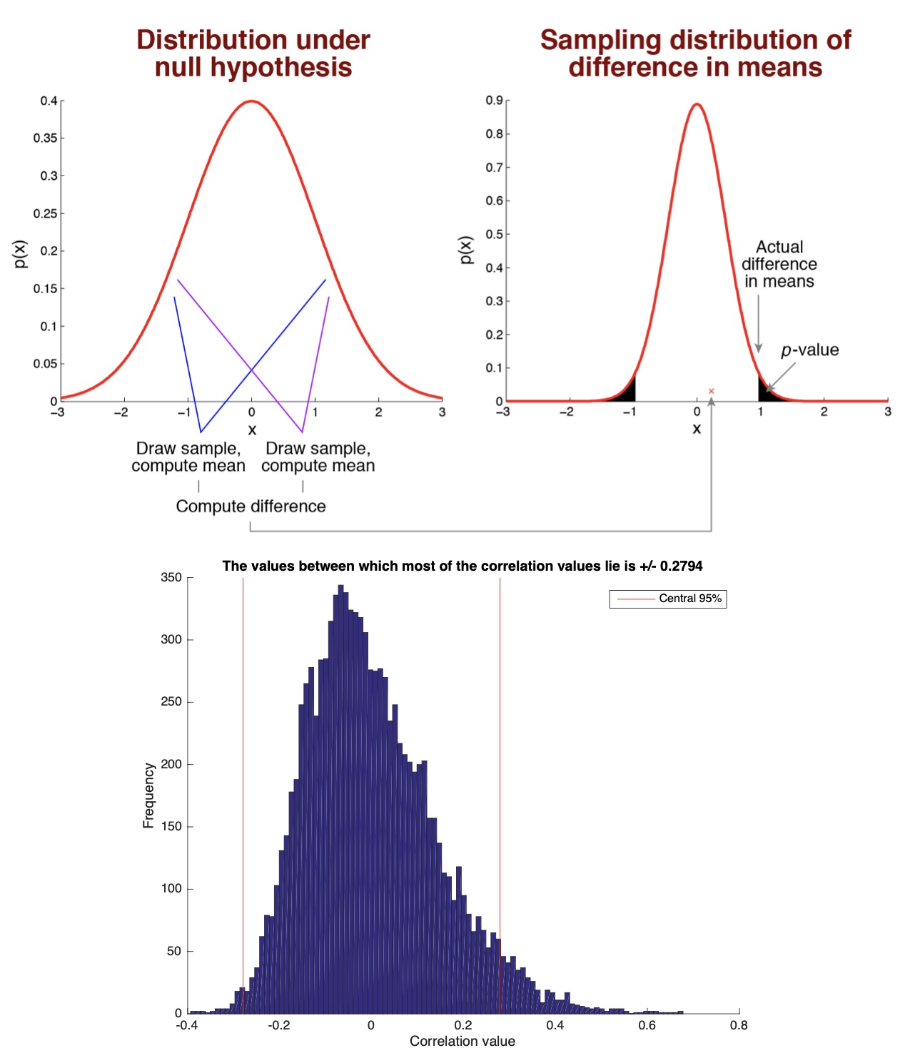
A small p-value (typically ≤ 0.05) indicates strong evidence against the null hypothesis, so you reject the null hypothesis. A large p-value (> 0.05) indicates weak evidence against the null hypothesis, so you fail to reject the null hypothesis. Here in our case, the p-value is 0.2794 so we fail to reject the null hypothesis.
MATLAB codes
clear; close all; clc;
% define
numsim = 10000; % number of simulations to run
samplesize = 50; % number of data points in each sample

data = (randn(samplesize,2).^2)*10+20;
% pre-allocate the results vector
results = zeros(1,numsim);

% loop over simulations
for num=1:numsim
  % draw two sets of random numbers, each from the normal distribution
  data = (randn(samplesize,2).^2)*10+20;
  % compute the correlation between the two sets of numbers and store the result
  results(num) = corr(data(:,1),data(:,2));
end

% visualize the results
figure;
hold on;
hist(results,100);
xlabel('Correlation value');
ylabel('Frequency');
%%
pval = prctile(abs(results),95)
%%

% visualize this on the figure
ax = axis;
h1 = plot([pval pval],ax(3:4),'r-');
h2 = plot(-[pval pval],ax(3:4),'r-');
legend(h1,'Central 95%');
title(sprintf('The values between which most of the correlation values lie is +/- %.4f',pval));
%%
MATLAB codes for wave propagation modeling
clear; close all; clc
% an illustration of a spherical wave
filename = 'wave_propagation.gif';
h=figure;
set(h,'color','w','Position',[440 122 350 1000])

plane_wave = 1;
spherical_wave = 2;

% wave_type = plane_wave;
wave_type = spherical_wave;

if wave_type == plane_wave

   % window size
   Lx=0.4;
   Ly=1;
   % blow up the image by this factor to display better
   factor = 80;

   % a small shift to be added below for graph. purposes.
   shift = .3;

elseif wave_type == spherical_wave

      Lx = 0.9;
      Ly=1.8;
%       Ly = Lx;
      factor = 5;
      shift = 5;
end

Mx = Lx/2;
Wy = Ly/2;

M=400;
N = floor(M*Ly/Lx);

% [X, Y]=meshgrid(linspace(-Lx/2, Lx/2, M), linspace(-Ly/2, Ly/2, N));
[X, Y]=meshgrid(linspace(0, Lx, M), linspace(-Ly, 0, N));
[Xr, Yr]=meshgrid(linspace(-Lx, 0, M), linspace(0, Ly, N));

wavenumber = 100;

T = 1;
nt = 20;
Time = linspace(0, T, nt);

for repeat = 1:1

   % go over one time period of the field
   for iter = 1:(nt-1) % nt is same as 1 due to peridicity

      t = Time(iter);

      if wave_type == plane_wave

         % plane wave
         Z = real(exp(i*wavenumber*Y)*exp(-i*2*pi*t));

      elseif wave_type == spherical_wave

         % spherical wave
         Z = exp(sqrt(-1)*wavenumber*sqrt(X.^2+Y.^2))*exp(-sqrt(-1)*2*pi*t)./sqrt(X.^2+Y.^2);
         Zr = exp(sqrt(-1)*wavenumber*sqrt(Xr.^2+Yr.^2))*exp(-sqrt(-1)*2*pi*t)./sqrt(Xr.^2+Yr.^2);

      end

      % plot the real part of the field Z

      figure(1); clf; hold on; axis equal; axis off;
      image(factor*(real(Z+Zr+shift))); % add shift to Z for graphing purposes
%       image(factor*(real(Zr+shift)));
      plot(7,788,'*r','MarkerSize',20)
      plot(400,3,'^r','MarkerSize',20)
      title('Wave propagation and Fresnels Zone')

      colormap jet; shading interp;
      drawnow
      frame = getframe(1);
      im = frame2im(frame);
      [A,map] = rgb2ind(im,256);
	if iter == 1;
		imwrite(A,map,filename,'gif','LoopCount',Inf,'DelayTime',1);
	else
		imwrite(A,map,filename,'gif','WriteMode','append','DelayTime',1);
	end
      file = sprintf('wave_frame%d.png', 1000+iter);
      disp(file); %show the frame number we are at
      print(file,'-dpng')
%       saveas(gcf, file, 'psc2') %save the current frame

      pause(0.1);

   end

end

% The following command was used to create the animated figure.
% convert -antialias -loop 10000  -delay 15 -compress LZW Movie_frame10* Spherical_wave2.gif
Disclaimer of liability
The information provided by the Earth Inversion is made available for educational purposes only.
Whilst we endeavor to keep the information up-to-date and correct. Earth Inversion makes no representations or warranties of any kind, express or implied about the completeness, accuracy, reliability, suitability or availability with respect to the website or the information, products, services or related graphics content on the website for any purpose.
UNDER NO CIRCUMSTANCE SHALL WE HAVE ANY LIABILITY TO YOU FOR ANY LOSS OR DAMAGE OF ANY KIND INCURRED AS A RESULT OF THE USE OF THE SITE OR RELIANCE ON ANY INFORMATION PROVIDED ON THE SITE. ANY RELIANCE YOU PLACED ON SUCH MATERIAL IS THEREFORE STRICTLY AT YOUR OWN RISK.
Leave a comment