Monte Carlo methods and earthquake location problem (codes included)
Introduction
In the last post, we looked into the introduction of the least-squares approach in geophysical inversion and we formulated a hypothetical earthquake location problem. We saw that we can simply invert for the solution: $\Delta m = (G^T G)^{-1} G^T \Delta d$. This is the simplest approach possible.
The common geophysical problems most often have multimodal objective function with many possible minima (solutions in simple words). Numerical algorithms such as steepest descent, Newton’s method, Quasi-Newton method, conjugate gradient method etc. (Kutz, 2013) tends to get trapped in the local minima if the initial parameters are not wisely chosen. Because of this reason, we seek some global search methods. In this post, we will look into the Monte Carlo methods to solve such problems.
Key idea — guess randomly, keep the best. Where least-squares slides downhill from a starting guess (and can slide into the wrong valley), Monte Carlo simply draws random models from the allowed parameter ranges, forward-models the arrival times each one predicts, scores the misfit against the observed data, and remembers the best model seen so far. Run enough draws and the best-so-far converges toward the global minimum. It shares the global-search robustness of a genetic algorithm but is even simpler: there is no population, no crossover, and no mutation — just draw, score, and keep.
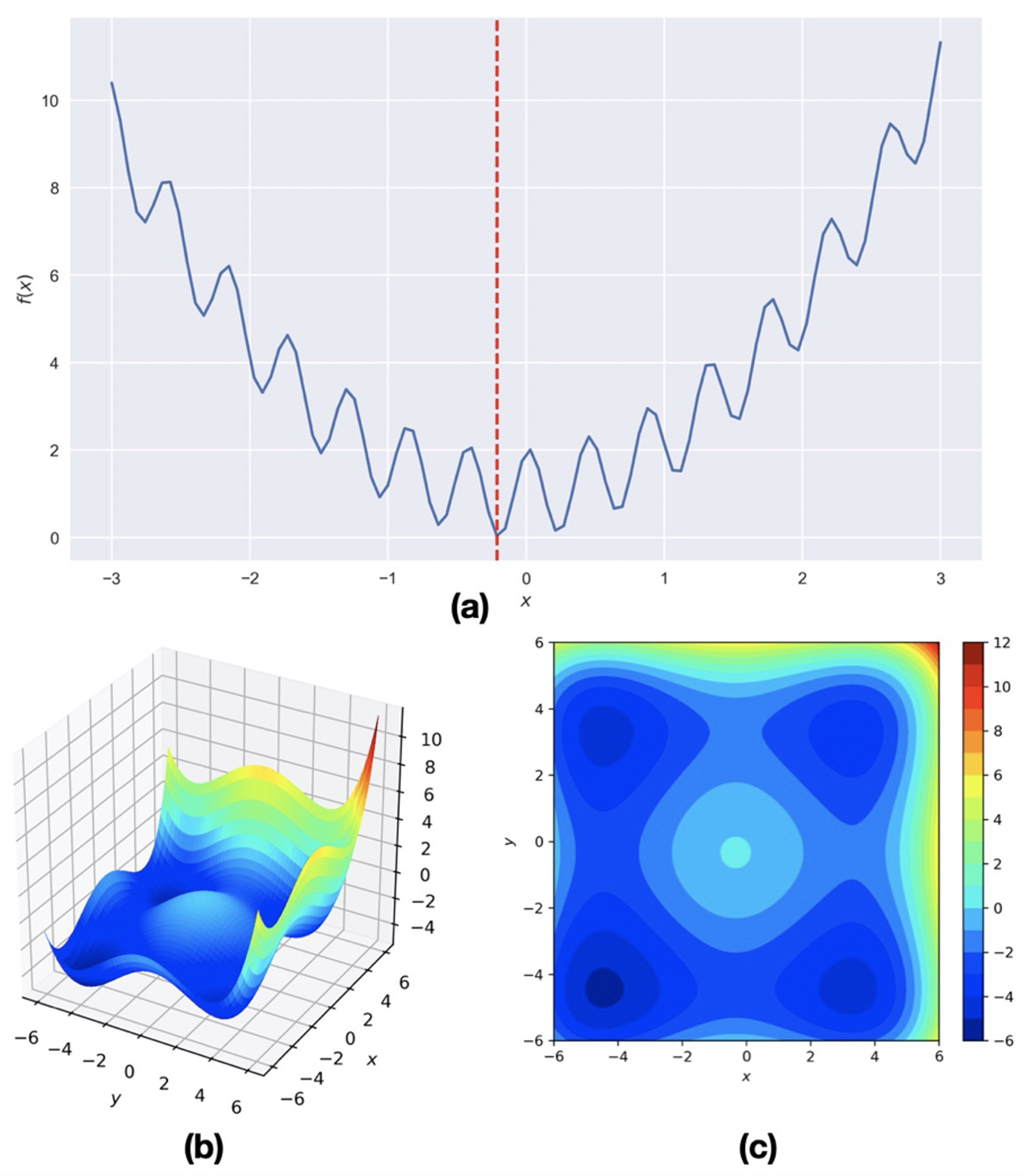
Figure 1: Hypothetical objective functions with global and local minima.
Monte Carlo Methods
Monte Carlo methods are widely used heuristic optimization technique. It makes clever sample from the parameter space to simulate the working of the complex system and aims to quickly converge for the optimal solution of the objective function. There are several flavors of Monte Carlo methods employed for different applications. The essence of Monte Carlo methods is the search for better sets of model parameters by iteratively generating random set of model parameters in each generation and computing for the least- squares error in the predicted and observed arrival times. The solution with the lowest least- squares error is the accepted solution.
Let us try to solve the earthquake location problem introduced in the previous post using the Monte Carlo method. The method is controlled mainly on two termination criteria - the maximum number of generations (or iterations) of the computation and the difference of the squared error obtained from the current set of model parameters and the squared error obtained from the previous best solution (tolerance value). If the least- squares errors in the predicted and observed arrival times at all the stations is less than the predefined tolerance value or the current generation number is equal to the predefined the number the maximum generations, the results are presented.
The least-squares error for this problem can be written as:
\[lse = \sum_{i=1}^{N} (d_i^{obs} - d_i^{pre})^2\]where N is the number of stations, $d_i^{obs}$ and $d_i^{pre}$ are the observed and predicted arrival times at each station.
The steps involved in Monte Carlo methods are:
- Define the termination criteria values: maximum number of iterations, and/or tolerance value.
- Define the lower and upper limits of the model parameters.
- Set the initial least-squares error value ($lse$). It is best to take it fairly large.
- Randomly generate the model parameters (earthquake coordinates, velocity and origin time) within the predefined limits (see Table 1)
- Compute the predicted arrival times at each station using the generated model parameters in step 4.
- Compute the $lse$ using the predicted arrival times for the current generation and the observed arrival times at each station
- If the error in the current generation is lower than the previous lowest $lse$, the best model parameters are updated using the current value.
- Steps 4-7 is repeated until any one of the termination criteria is satisfied.
- Once the termination criteria are satisfied, the best model parameters are presented.
Table 1: Lower and upper limits of the model parameters for the Monte Carlo solution to earthquake location problem
| Model Parameter | Min Value | Max Value |
|---|---|---|
| Earthquake x-coordinate | -3 | 3 |
| Earthquake y-coordinate | -3 | 3 |
| Earthquake z-coordinate | -3 | 0 |
| Velocity | 5 | 7 |
| Origin Time | -1 | 1 |
I made the maximum generations to be fairly large (100,000) and the tolerance value as $10^3$. The model parameters value at each generation are generated randomly within the predefined range (see Table 1). The obtained best model parameters solution is [2.34, 2.30, -1.94, 6.37, -0.01].
Import libraries
import matplotlib.pyplot as plt
import numpy as np
import pandas as pd
from mpl_toolkits.mplot3d import Axes3D
from matplotlib import cm

np.random.seed(0)

plt.style.use('seaborn')
Two small updates for a current environment. plt.style.use('seaborn') was removed in matplotlib 3.8 — use plt.style.use('seaborn-v0_8') instead (or import seaborn as sns; sns.set_theme()). The np.random.seed(0) / np.random.rand / np.random.uniform calls below still work, but NumPy now recommends the generator API — rng = np.random.default_rng(0) then rng.random(...), rng.uniform(...) — for new code. The results and logic here are unchanged either way.
Set up stations to record earthquake
minx, maxx = -2, 2
miny, maxy = -3, 3
numstations = 30
stn_locs=[]
xvals = minx+(maxx-minx)*np.random.rand(numstations)
yvals = miny+(maxy-miny)*np.random.rand(numstations)

for num in range(numstations):
    stn_locs.append([xvals[num],yvals[num],0])
Set up the earthquake
eq_loc = [2,2,-2]
vel = 6 #kmps
origintime = 0

def calc_arrival_time(eq_loc, stnx, stny, stnz, vel, origintime):
    eqx, eqy, eqz = eq_loc
    dist = np.sqrt((eqx - stnx)**2 + (eqy - stny)**2 + (eqz - stnz)**2)
    arr = dist/vel + origintime
    return arr
Make the earthquake arrivals noisy
d_obs = []
noise_level_data = 0.001
for stnx, stny, stnz in stn_locs:
    arr = calc_arrival_time(eq_loc, stnx, stny, stnz, vel, origintime)
    sign = np.random.choice([-1,1])
    d_obs.append(arr+sign*noise_level_data*arr)

d_obs = np.array(d_obs)
Monte Carlo Solution
def get_rand_number(min_value, max_value):
    range_vals = max_value - min_value
    choice = np.random.uniform(0,1)
    return min_value + range_vals*choice

## Monte Carlo

num_iterations = 100000
inv_model = []
squared_error0 = 100000

mineqx, maxeqx = -3, 3
mineqy, maxeqy = -3, 3
mineqz, maxeqz = 0, -3
gen_num = []
lse = []
for i in range(num_iterations):
    eqx0 = get_rand_number(mineqx, maxeqx)
    eqy0 = get_rand_number(mineqy, maxeqy)
    eqz0 = get_rand_number(mineqz, maxeqz)
    vel0 = get_rand_number(5, 7)
    origintime0 = get_rand_number(-1, 1)
    d_pre = []
    for stnx, stny, stnz in stn_locs:
        d_pre.append(calc_arrival_time([eqx0, eqy0, eqz0], stnx, stny, stnz, vel0, origintime0))
    d_pre = np.array(d_pre)

    squared_error = np.sum((d_obs-d_pre)**2)
    if squared_error < squared_error0:
        print(i,squared_error)
        gen_num.append(i)
        lse.append(squared_error)
        m0 =  np.array([eqx0, eqy0, eqz0, vel0, origintime0])
        if np.abs(squared_error-squared_error0)<0.001:
            print("Terminated based on tol. value",np.abs(squared_error-squared_error0))
            break
        squared_error0 = squared_error
        inv_model = m0

print("{:.2f} {:.2f} {:.2f} {:.2f} {:.2f}".format(inv_model[0],inv_model[1],inv_model[2],inv_model[3],inv_model[4]))
Plot least squares error corresponding to each generations
fig, ax = plt.subplots(1,1,figsize=(5,5))
ax.loglog(gen_num,lse, 'ko--')
ax.set_xlabel('Generations')
ax.set_ylabel('Least-squares error')
plt.savefig('iterations.png',bbox_inches='tight',dpi=300)
plt.close('all')
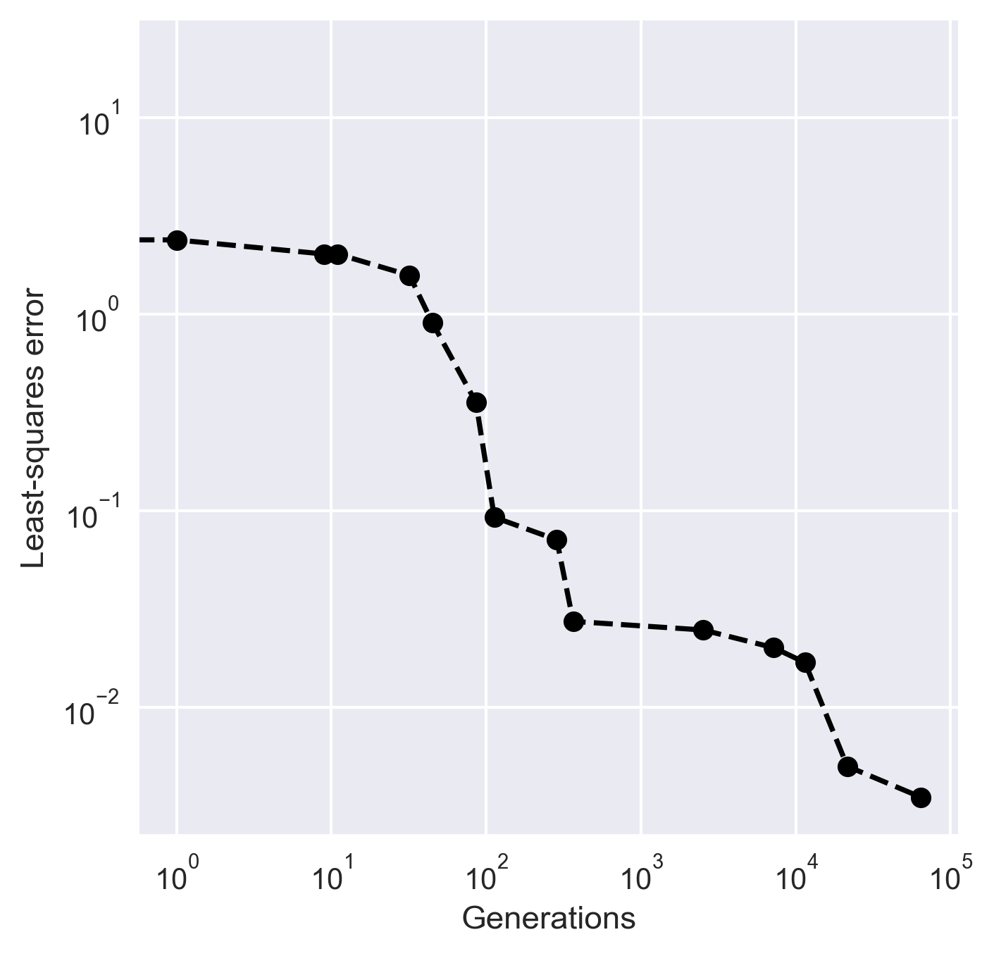
Figure 2:The convergence of least-squares error to find the best model parameters
Plot the solution
## to create the surface
X = np.linspace(-3, 3, 200)
Y = np.linspace(-3, 3, 200)
X, Y = np.meshgrid(X, Y)
Z = (X**2 + Y**2)*0

fig = plt.figure()
ax = plt.axes(projection='3d')
# plot stations
ax.scatter([x[0] for x in stn_locs],[x[1] for x in stn_locs],[x[2] for x in stn_locs],c='b',marker='^',s=50)
# plot surface
surf = ax.plot_surface(X, Y, Z, rstride=1, cstride=1, cmap=cm.jet,linewidth=0, antialiased=False,alpha=0.1)
# plot actual EQ
ax.scatter(eq_loc[0],eq_loc[1],eq_loc[2],c='r',marker='*',s=100,label='Actual EQ location')
ax.scatter(inv_model[0],inv_model[1],inv_model[2],c='k',marker='*',s=100,label='Inverted EQ location')
plt.title("Inverted model EQ loc: ({:.2f},{:.2f},{:.2f}),\nvel: {:.2f} and origin time: {:.2f}\nsq_error: {:.2f}".format(inv_model[0],inv_model[1],inv_model[2],inv_model[3],inv_model[4],squared_error),fontsize=8)
ax.set_xlim([-3,3])
ax.set_ylim([-3,3])
ax.set_zlim(-3,0.1)
plt.legend()

plt.savefig('Earthquake_loc_monte_carlo.png',bbox_inches='tight',dpi=300)
plt.close('all')
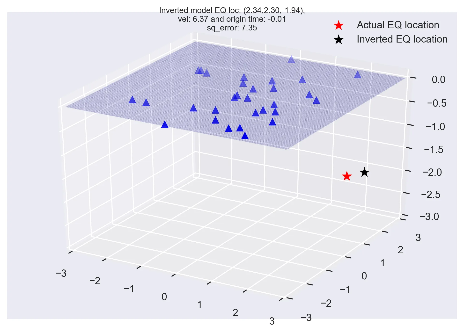
Figure 3: Hypothetical earthquake location solution using Monte Carlo method.
The actual earthquake location is (2,2,-2), velocity of the homogeneous medium is 6 unit/s, and the actual origin time is 0s. The location of the 30 stations and the actual and inverted earthquake location.
Quick check: Why does a Monte Carlo search succeed on a multi-modal misfit surface where a steepest-descent method might fail?
- It computes the exact analytical minimum in one step
- It samples the whole parameter space at random, so it is not tied to a single starting point that could sit in the wrong local valley
- It needs the misfit function to be smooth and differentiable
- It always finds the answer in fewer iterations than any other method
Recap
- The earthquake-location misfit is multi-modal, so local methods (steepest descent, Newton) can converge to the wrong minimum depending on the starting guess.
- Monte Carlo sidesteps that by random global sampling: draw a model within bounds, forward-model the arrival times, score the least-squares misfit $\sum (d^{obs}_i - d^{pre}_i)^2$, and keep the best model seen so far.
- Two termination criteria stop the loop: a maximum number of iterations (here 100,000) and a tolerance on the change in misfit.
- It is simpler than a genetic algorithm — no population, crossover, or mutation — at the cost of not reusing information from good samples, so it can need many draws.
- Being random, it is stochastic: fixing the seed (
np.random.seed(0)) makes a run reproducible, and averaging several runs gives a more stable estimate.
Where to go next
- The earthquake location problem and the least-squares method — the local baseline this post improves on.
- An introduction to the genetic algorithm — a smarter global search that evolves good samples instead of discarding them.
- Solving a toy earthquake-location problem using a genetic algorithm — a hands-on Python walkthrough of the same problem.
Disclaimer of liability
The information provided by the Earth Inversion is made available for educational purposes only.
Whilst we endeavor to keep the information up-to-date and correct. Earth Inversion makes no representations or warranties of any kind, express or implied about the completeness, accuracy, reliability, suitability or availability with respect to the website or the information, products, services or related graphics content on the website for any purpose.
UNDER NO CIRCUMSTANCE SHALL WE HAVE ANY LIABILITY TO YOU FOR ANY LOSS OR DAMAGE OF ANY KIND INCURRED AS A RESULT OF THE USE OF THE SITE OR RELIANCE ON ANY INFORMATION PROVIDED ON THE SITE. ANY RELIANCE YOU PLACED ON SUCH MATERIAL IS THEREFORE STRICTLY AT YOUR OWN RISK.
Leave a comment