High-quality maps using the modern interface to the Generic Mapping Tools (codes included)
GMT or generic mapping tools have become synonymous with plotting maps in Earth, Ocean, and Planetary sciences. It can be used for processing data, generating publication-quality illustrations, automating workflows, and even making awesome animations. Another great thing about GMT is that it supports many map projections and transformations and includes supporting data such as coastlines, rivers, and political boundaries, and optionally country polygons.

One of the favorite parts of working in geophysics is without a doubt creating amazing visualizations. Visualizations are the best tool to effectively convey our findings to the scientific community.
GMT or generic mapping tools have become synonymous with plotting maps in Earth, Ocean, and Planetary sciences. It can be used for processing data, generating publication-quality illustrations, automating workflows, and even making awesome animations. Another great thing about GMT is that it supports many map projections and transformations and includes supporting data such as coastlines, rivers, and political boundaries, and optionally country polygons.
I have talked about GMT 5 and how to use it to plot high-quality maps in multiple posts. I have also talked about the Python interface to GMT 6 - the PyGMT in detail. The PyGMT uses GMT 6 under the hood to do all the tasks.
In this post, my goal is to introduce you to the basics of using GMT 6 for creating simple maps and get you familiar with the syntax. Most of the styles in GMT 6 are almost the same as the GMT 5 except the coding syntax has been improved significantly. It has become much more organized and can perform more with fewer codes. It has added the option to use meaningful full commands rather than simply its aliases. It will become more clear when we discuss this with some examples.
Install GMT
For installing GMT you can follow the steps from here Install the required software.
I use Ubuntu (as Windows Subsystem - WSL), so I can simply install using conda package manager. See this. The steps are similar for any Linux or Unix operating system.
Our codes will be written in bash. I am here assuming that you have a basic understanding of bash. But even if you are not much familiar with bash, you can still follow along as I will try to make the script “ready for production”, so that you don’t have to learn much to accomplish the tasks covered in this tutorial.
First Look
The first thing different with GMT 6 is the following syntax:
gmt begin [session-name] [graphics-formats]
	<LIST OF COMMANDS>
gmt end [show]
The above syntax only works with GMT6 and is not backward compatible. So, you will not be accidentally running the GMT version < 6. GMT session starts with gmt begin and ends with gmt end. Optionally, you can provide the name of the session that will be used for the output if you give the output format as graphics-formats. If you don’t provide the session-name or the graphics-formats, then the defaults will be used. The plot will not be saved but instead only displayed if you gave the option of show at the gmt end.
If you want to quickly look into the documentation, you can do that by typing
gmt docs [command name]
This will open the local GMT docs file, so you don’t need internet.
First Plot
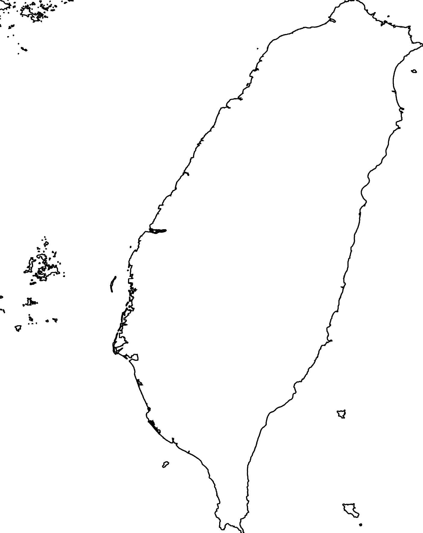
gmt begin taiwan pdf,png
    gmt coast -RTW -Wthin
gmt end
The above script plots a coastline map of Taiwan with the thick coastline thickness and saves it in a pdf and png formats. The png is the raster image format and is asked by the journals for publication. If you want a vector image, pdfgives the vector format. Other vector formats such as ps or eps, etc are also supported.
We can add the default frame to the plot by using -B option. We may also like to offset the figure a bit from the frame border. We can achieve a quick offset by simply specifying +r0.5 to the -RTW to tell GMT to offset the Taiwan map by 0.5 degrees.
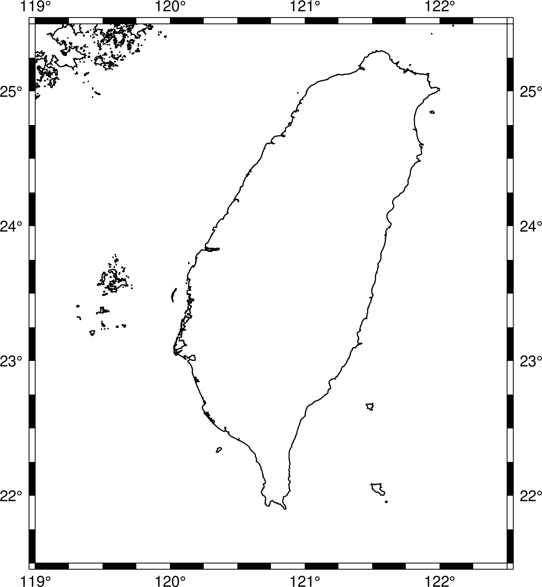
We can get the same above plot by simply specifying the map borders instead of using TW as the region. This gives us more control on plotting.
gmt begin taiwan pdf,png
    gmt coast -R119/122.5/21.5/25.5 -Wthin -B
gmt end
Here, you might have noticed that we have not specified any projection of the Map. The above plot uses the default projection for plotting. In science, for most of the practical purposes, we use the Mercator projection. To use the Mercator projection, we can tell GMT that we want it by -JM and then we can specify the width of the map, -JM15c for instance for a 15cm map.
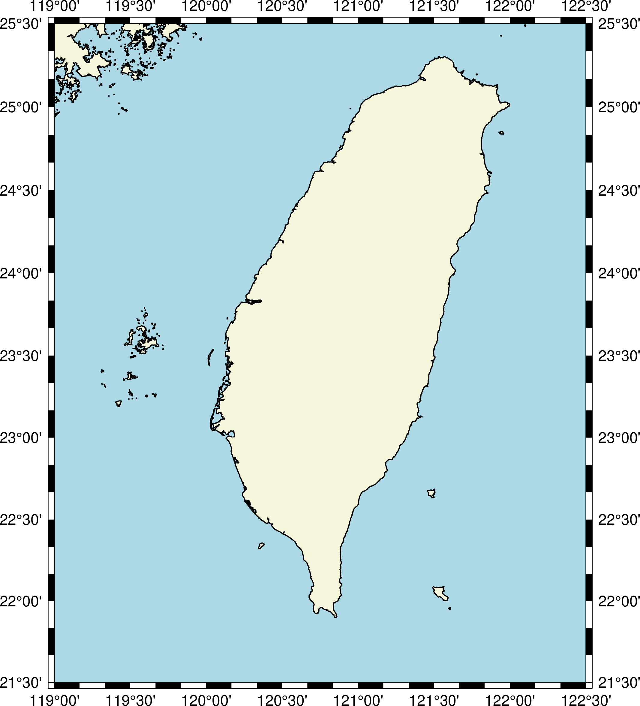
Fill the colors to land and water
Next, we can fill some colors to the map to make it more attractive.
gmt begin taiwan png
    gmt coast -R119/122.5/21.5/25.5 -Wthin -B -JM15c -Gbeige -Slightblue
gmt end
We specified the land color by -G and the watercolor by -S. You can look for more colors in the get colors list. Simply run the command gmt docs gmt colors.
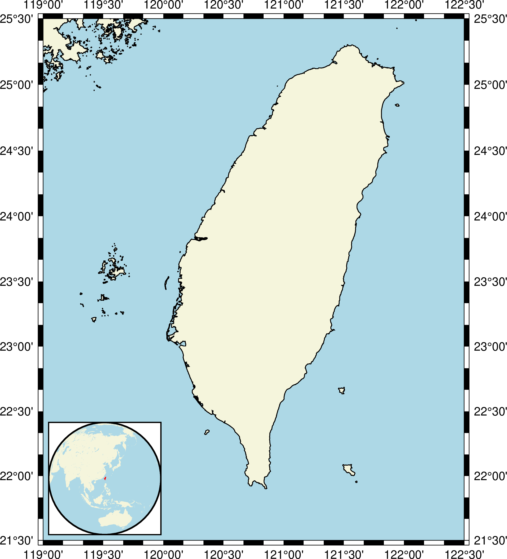
Inset to the map
Now, let us try to plot another map on top of the above plot as an inset. I want to put the inset at the top-left corner of the map with a width of 4cm. In the inset, I want to show Taiwan on a world map.
gmt begin taiwan png
    gmt coast -R119/122.5/21.5/25.5 -Wthin -B -JM15c -Gbeige -Slightblue
    gmt inset begin -DjBL+w4c+o0.2c -M0 -F+gwhite+pthick
        gmt coast -Rg -JG120.5/23.5/4c -Gbeige -Slightblue -B -ETW+gred
    gmt inset end
gmt end
Let us go through each part of the above code. We begin the inset figure by using the “context manager” gmt inset begin and we end it at the end of the inset sub-part of the script. We specified using -Dj that we want to use the justification method to specify the location of the inset and we set the location to be “bottom-left” (BL) corner. We want the map of width 4cm and of offset 0.2 cm. Further, we specified that we want no margin (M0) and the background of the frame to be white and frame border with the thick lines.
We plot the coastline map inside the inset in the same way we did before. Additionally, we told GMT to highlight Taiwan with the red color (-ETW+gred).
Subplots in GMT
Now, let us see how we can use GMT to make the figure with multiple subplots.
#!/bin/bash
gmt begin subplotMap png
    gmt subplot begin 2x2 -Ff16c/25c -M0 -A
    #figure a
    gmt coast -R119/122.5/21.5/25.5 -BNWse -Wthin -Gbeige -Slightblue

    #figure b
    gmt coast -R119/122.5/21.5/25.5 -BswNE -Wthin -Gbeige -Slightblue -c
    gmt grdcontour @earth_relief_01m -Wared -Wcthinnest,blue -C1000 -A2000 #contour every 1000m, annotation every 2000 m

    #figure c
    gmt coast -R119/122.5/21.5/25.5 -BnWSe -Wthin -Gbeige -Slightblue -c
    gmt grdcontour @earth_relief_01m -LP -Wared -C1000 -A2000 #contour every 1000m, annotation every 2000 m
    gmt grdcontour @earth_relief_01m -Ln -Wablue -C2000 -A4000 #contour every 2000m, annotation every 4000 m

    #figure d
    gmt coast -R119/122.5/21.5/25.5 -BSwne -Wthin -Gbeige -Slightblue -c
    gmt makecpt -Cabyss -T-10000/0
    gmt coast -Sc #clip out the land part
    gmt grdimage @earth_relief_01m -C -I+d #+d for default gradient for shadow
    gmt coast -Q #terminate clipping
    gmt colorbar -DJBC -B2000
    gmt makecpt -Cgeo -T0/5000
    gmt coast -Gc #clip out the water part
    gmt grdimage @earth_relief_01m -C -I+d #+d for default gradient for shadow
    gmt coast -Q #terminate clipping
    gmt colorbar -DJRR -B1000
    gmt subplot end
gmt end
Let us go through the above script now.
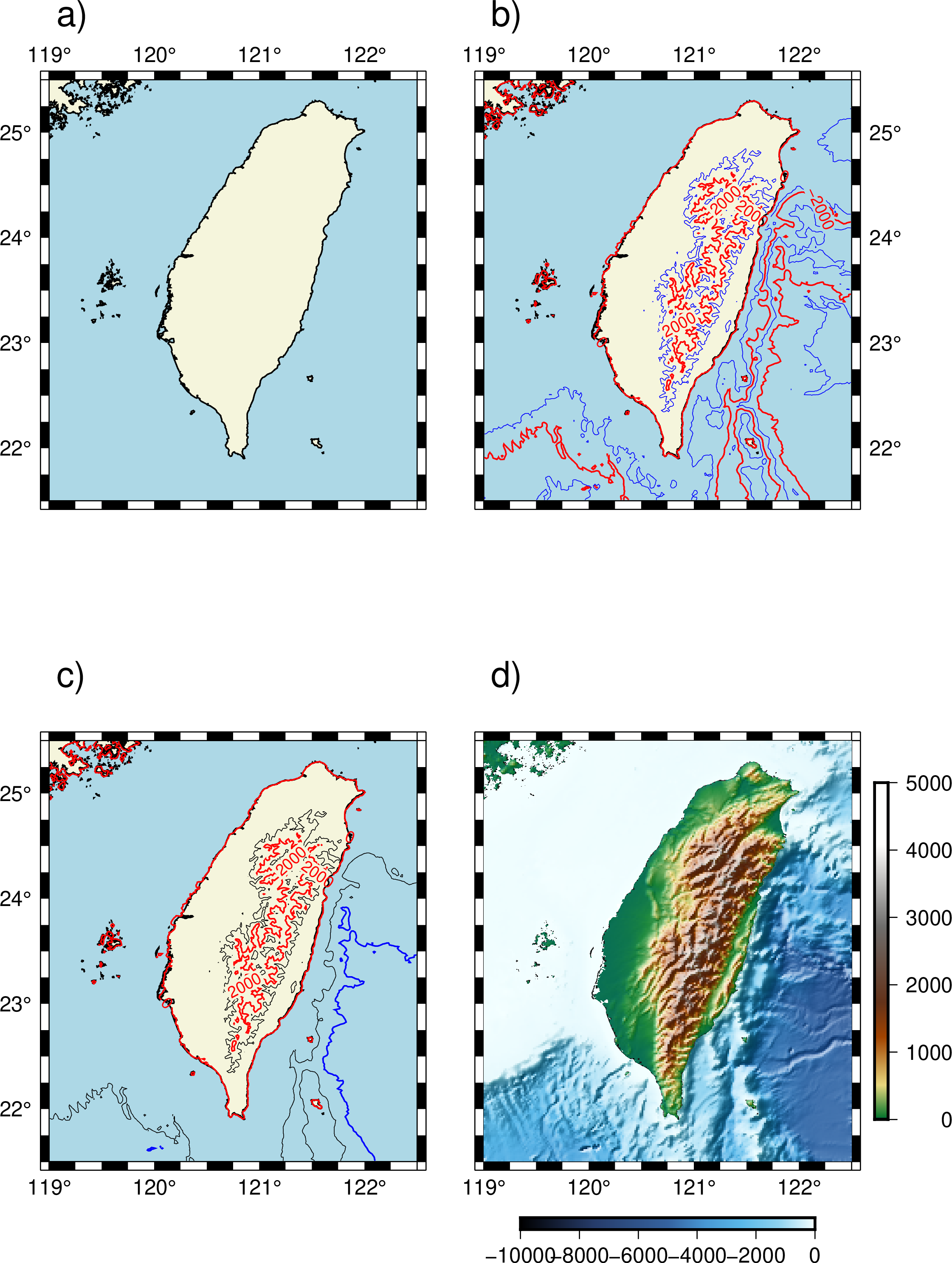
I plotted the subplots with 4 subplots (2 x 2). I can specify that by simply typing 2x2. The dimension of each subplot is specified by the argument -Ff16c/25c. We ask each subplot to be 16cm wide by 25cm long. By argument -A, we asked GMT to automatically annotate the subplots. Navigation to the next subplot can be specified using the -c argument.
Next, I made four figures in the subplots.
Figure (a) is simply what we did in the previous section but here we put the tick marks only on the top and left side.
In the figure (b), we plotted the contour lines for topography of resolution 1m. We plotted the annotated contour lines with the red color and the regular ones with the blue color. The regular contour lines is made to be plotted with the thinnest line widths. The contour lines are plotted for every 1000m and the annotation is done for every 2000m.
In the figure (c), we separated the contour lines plotting for the land and the sea part. This can be simply specified with the argument -L followed by P or N. P is for positive and N is for negative. The upper case is inclusive of 0 and vice-versa. So, we plotted the positive annotated contour lines with red and the negative ones with the blue color.
In figure (d), we plot the topographic map with two colorbars. For this figure also, we start with the coast lines (note that this is not required, you can simply jump to the next step). Then we created our custom colormap based on abyssstandard colormap but specified the range between -10000 to 0. Then we clip out the land part and did the plotting for the sea part. Next, we did the same by clipping out the sea part and we plotted the land part with different colormap. Finally, we plot the colorbar for the both land and sea part separately, one at the bottom-center and the other at the right corner.
Conclusions
There is a lot more one can do with GMT. I will try to cover that in the future posts. For more GMT related examples, you can look at the other posts in my blog. I hope this tutorial will come handy in your endeavors.
References
Disclaimer of liability
The information provided by the Earth Inversion is made available for educational purposes only.
Whilst we endeavor to keep the information up-to-date and correct. Earth Inversion makes no representations or warranties of any kind, express or implied about the completeness, accuracy, reliability, suitability or availability with respect to the website or the information, products, services or related graphics content on the website for any purpose.
UNDER NO CIRCUMSTANCE SHALL WE HAVE ANY LIABILITY TO YOU FOR ANY LOSS OR DAMAGE OF ANY KIND INCURRED AS A RESULT OF THE USE OF THE SITE OR RELIANCE ON ANY INFORMATION PROVIDED ON THE SITE. ANY RELIANCE YOU PLACED ON SUCH MATERIAL IS THEREFORE STRICTLY AT YOUR OWN RISK.