Locating Earthquakes using Geiger’s Method (codes included)
Introduction
The earthquake location problem is old; however, it is still quite relevant. The problem can be stated as to determine the hypocenter ($x_0$, $y_0$, $z_0$) and origin time ($t_0$) of the rupture of fault based on arrival time data of P and S waves. Here, we have considered a hypocenter in the cartesian coordinate system. It can be readily converted to geographical coordinates using an appropriate conversion factor. The origin time is the start time of the fault rupture.
Key idea — guess, linearize, correct, repeat. The travel-time equation is non-linear in the hypocenter, so there’s no one-shot formula. Geiger’s method turns it into a sequence of linear steps: start from a trial hypocenter, predict the arrival times, measure the residuals (observed − predicted), linearize the travel times about the current guess to build the kernel $G$ of partial derivatives, then solve a damped least-squares system for a small correction $\Delta m$ and update the guess. Iterate until the residuals stop shrinking. It’s Gauss–Newton on the arrival-time misfit — fast when the starting guess is decent, but it can settle into a local minimum, which is why the damping term and a sensible initial guess matter.
Determine the hypocenter and origin time
Here, our data are the P and S arrival times at the stations located at the surface ($x_i$, $y_i$, 0). We have also assumed a point source and a constant velocity medium for the simplicity sake.
The arrival time of the P or S wave at the station is equal to the sum of the origin time of the earthquake and the travel time of the wave to the station.
The arrival time, $t_i = T_i + t_0$, where $T_i$ is the travel time of the particular phase and $t_0$ is the origin time of the earthquake.
\[\begin{aligned} T_i = \sqrt{((x_i-x_0)^2 + (y_i-y_0)^2 + z_0^2)/v} \end{aligned}\]Where v is the P or S wave velocity.
Now, we have to determine the hypocenter location and the origin time of the Earthquake. This problem is invariably ill-posed as the data are contaminated by noise. So, we can pose this problem as an over-determined case. One way to solve this inconsistent problem for the hypocenter and origin time is to minimize the least square error of the observed and predicted arrival times at the stations.
Before that, we need to formulate the problem. As evident from the above equation, the expression for arrival time and eventually the least square error function is nonlinear. This nonlinear inverse problem can be solved using the Newton’s method. We will utilize the derivative of the error function in the vicinity of the trial solution (initializing the problem with the initial wise guess) to devise a better solution. The next generation of the trial solution is obtained by expanding the error function in a Taylor series about the trial solution. This process continues until the error function becomes considerably small. Then we accept that trial solution as the estimated model parameters.
$d = G m$, where d is the matrix containing the arrival time data, m is the matrix containing the model parameters, and G is the data kernel which maps the data to the model.
There are some instances where the matrix can become underdetermined and the least square would fail such as when the data contains only the P wave arrival times. In such cases the solution can become nonunique. We solve this problem as a damped least square case. Though it can also be using the singular value decomposition which allows the easy identification of the underdetermined case and then partitioning the overdetermined and underdetermined in upper and lower part of the kernel matrix and dealing with both part separately.
\[\begin{aligned} m = [G'G + \epsilon]G'd \end{aligned}\]The parameter epsilon is chosen by trial and error to yield a solution that has a reasonably small prediction error.
In this problem, we deduce the gradient of the travel time by examining the geometry of the ray as it leaves the source. If the earthquake is moved a small distance s parallel to the ray in the direction of the receiver, then the travel time is simply decreased by $s/v$, where v is the velocity of the phase. If the earthquake is moved a small distance perpendicular to the ray, then the change in travel time is negligible since the new path will have nearly same length as the old one.
\[\begin{aligned} T = \frac{r}{v} \end{aligned}\]If the earthquake is moved parallel to the ray path,
\[\begin{aligned} T'' &= \frac{(r-s)}{v} = \frac{r}{v} - \frac{s}{v}\\ \delta T = T'' - T &= \frac{r}{v} - \frac{s}{v} - \frac{r}{v} = - \frac{s}{v} \end{aligned}\]If the earthquake has moved perpendicular to the raypath,
\[\begin{aligned} \delta T = 0 \end{aligned}\]So, $\delta T = - s/v$, where s is a unit vector tangent to the ray at the source and points toward the receiver.
This is the Geiger’s Method, which is used to formulate the data kernel matrix.
Example hypothetical earthquake location problem
Let us take a hypothetical earthquake location problem and solve it using this method.
Defining the region of the problem
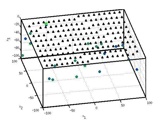
Let us define the region of the problem which contains both the source and the receiver. We take a 100x100 units^2 area and the depth of 100 units. The surface is 0 units depth.
clear; close all;
global G epsilon;
epsilon=1.0e-6;

% Velocity parameters
vpvs = 1.78;
vp=6.5;
vs=vp/vpvs;

% defining the region of the problem which contains both the source and the receiver
%We take a 100x100 units^2 area and the depth of 100 units. The surface is 0 units depth.
xmin=-100;
xmax=100;
ymin=-100;
ymax=100;
zmin=-100;
zmax=0;

% stations: x, y, z coordinates (xi, yi, 0)
sxm = [-9, -8, -7, -6, -5, -4, -3, -2, -1, 0, 1, 2, 3, 4, 5, 6, 7, 8, 9]'*ones(1,9)*10;
sym = 10*ones(9,1)*[-9, -8, -7, -6, -5, -4, -3, -2, -1, 0, 1, 2, 3, 4, 5, 6, 7, 8, 9];
sx = sxm(:);
sy = sym(:);
Ns = length(sx); % num of stations
sz = zmax*ones(Ns,1); %zeros
Define true earthquake location
% true earthquakes locations
Ne = 20; % number of earthquakes
M = 4*Ne; % 4 model parameters, x, y, z, and t0, per earthquake
extrue = random('uniform',xmin,xmax,Ne,1); %x0
eytrue = random('uniform',ymin,ymax,Ne,1); %y0
eztrue = random('uniform',zmin,zmax,Ne,1); %z0
t0true = random('uniform',0,0.2,Ne,1); %t0
mtrue = [extrue', eytrue', eztrue', t0true']'; %column matrix containing all the true model parameter values

Nr = Ne*Ns; % number of rays, that is, earthquake-stations pairs
N = 2*Ne*Ns; % total data; Ne*Ns for P and S each
Generating synthetic data
We generate the true data based on the true earthquake and station locations
% Generating the true data based on the true earthquake and station locations
dtrue=zeros(N,1); %allocating space for all data
for i = [1:Ns] % loop over stations
  for j = [1:Ne] % loop over earthquakes
    dx = mtrue(j)-sx(i); % x component of the displacement obtained by the difference between station and source location x component
    dy = mtrue(Ne+j)-sy(i); % y component of the source- receiver displacement
    dz = mtrue(2*Ne+j)-sz(i); % z component of displacement between source and receiver
    r = sqrt( dx^2 + dy^2 + dz^2 ); % source-receiver distance
    k=(i-1)*Ne+j;
    dtrue(k)=r/vp+mtrue(3*Ne+j); %P arrival time for each station-source pair obtained by summing the travel time with the origin time of the earthquake
    dtrue(Nr+k)=r/vs+mtrue(3*Ne+j); % S arrival time
  end
end
Next, we create observed data from the true data by adding some random noise.
%  Generating observed data by adding gaussian noise with standard deviation 0.2
sd = 0.2;
dobs=dtrue+random('normal',0,sd,N,1); % observed data
And, predicted arrival times
%% Determining the predicted arrival time using the Geiger's Method
% inital guess of earthquake locations
mest = [random('uniform',xmin,xmax,1,Ne), random('uniform',ymin,ymax,1,Ne), ...
 random('uniform',zmin+2,zmax-2,1,Ne), random('uniform',-0.1,0.1,1,Ne) ]';
% Here, we take a random initial guess
Formulating data kernel and estimating predicted models
We will solve the damped least squares equation using the biconjugate method to reduce the cost function.
%Formulating the data kernel matrix and estimating the predicted models
for iter=[1:10] %for 10 iterations (termination criteria)

  % formulating data kernel
  G = spalloc(N,M,4*N); %N- total num of data,2*Ne*Ns; M is total num of model
  %parameters, 4*Ne
  dpre = zeros(N,1); %allocating space for predicted data matrix
  for i = 1:Ns % loop over stations
  for j = 1:Ne % loop over earthquakes
  dx = mest(j)-sx(i); % x- component of displacement obtained using the initial guess
  dy = mest(Ne+j)-sy(i); % y- component of displacement
  dz = mest(2*Ne+j)-sz(i); % z- component of displacement
  r = sqrt( dx^2 + dy^2 + dz^2 ); % source-receiver distance for each iteration
  k=(i-1)*Ne+j; %index for each ray
  dpre(k)=r/vp+mest(3*Ne+j); %predicted P wave arrival time
  dpre(Nr+k)=r/vs+mest(3*Ne+j); %predicted S wave arrival time
  %First half of data kernel matrix correspoding to P wave
  G(k,j) = dx/(r*vp); % first column of data kernel matrix
  G(k,Ne+j) = dy/(r*vp); % second column of data kernel matrix
  G(k,2*Ne+j) = dz/(r*vp); % third column of data kernel matrix
  G(k,3*Ne+j) = 1; % fourth column of data kernel matrix
  % Second half of the data kernel matrix corresponding to S wave
  G(Nr+k,j) = dx/(r*vs);
  G(Nr+k,Ne+j) = dy/(r*vs);
  G(Nr+k,2*Ne+j) = dz/(r*vs);
  G(Nr+k,3*Ne+j) = 1;
  end
 end

 % solve with dampled least squares
 dd = dobs-dpre;
 dm=bicg(@dlsfun,G'*dd,1e-5,3*M); %solving using the biconjugate method
%solving the damped least square equation G'dd = [ G'G + epsilon* I] dm
% We use biconjugate method to reduce the computational cost (see for the dlsfun at the bottom)
 mest = mest+dm; %updated model parameter

end
Generating estimated data from the predicted model
% Generating the final predicted data
dpre=zeros(N,1);
for i = 1:Ns % loop over stations
for j = 1:Ne % loop over earthquakes
 dx = mest(j)-sx(i);
 dy = mest(Ne+j)-sy(i);
 dz = mest(2*Ne+j)-sz(i);
 r = sqrt( dx^2 + dy^2 + dz^2 );
 k=(i-1)*Ne+j;
 dpre(k)=r/vp+mest(3*Ne+j); % S-wave arrival time
 dpre(Nr+k)=r/vs+mest(3*Ne+j); % P- wave arriavl time
end
end
Calculate the data and model misfit
% Calculating the data and model misfit
expre = mest(1:Ne); % x0
eypre = mest(Ne+1:2*Ne); %y0
ezpre = mest(2*Ne+1:3*Ne); %z0
t0pre = mest(3*Ne+1:4*Ne); %t0
dd = dobs-dpre; %residual of observed and predicted arrival time
E = dd'*dd; %error
fprintf('RMS traveltime error: %f\n', sqrt(E/N) );
Emx = (extrue-expre)'*(extrue-expre); %misfit for x0
Emy = (eytrue-eypre)'*(eytrue-eypre); %misfit for y0
Emz = (eztrue-ezpre)'*(eztrue-ezpre); %misfit for z0
Emt = (t0true-t0pre)'*(t0true-t0pre); %misfit for t0
fprintf('RMS model misfit: x %f y %f z %f t0 %f\n', sqrt(Emx/Ne), sqrt(Emy/Ne), sqrt(Emz/Ne), sqrt(Emt/Ne) );
Support Function
dlsfun.m:
function y = dlsfun(v,transp_flag)
global G epsilon;
temp = G*v;
y = epsilon * v + G'*temp;
return
Quick check: Why does Geiger’s method iterate rather than solve the hypocenter in a single step?
- Because computers are too slow to solve it once
- Because the travel-time equations are non-linear, so each step only solves a linearized approximation and must be repeated as the guess improves
- Because it needs a new set of stations each iteration
- Because the origin time is unknown
Recap
- Geiger’s method locates an earthquake by minimizing the misfit between observed and predicted P/S arrival times — a non-linear least-squares problem.
- It works by linearizing the travel times about a trial hypocenter (the kernel $G$ holds $\partial t/\partial m$), solving for a correction $\Delta m$, updating the guess, and iterating — Gauss–Newton.
- Moving the source along the ray changes the travel time by $\delta T = -s/v$; moving it perpendicular to the ray barely changes it — that geometry is the kernel.
- Using only P arrivals can make the problem under-determined; a damped least-squares term ($\epsilon$) keeps the solution stable, and the biconjugate-gradient solver keeps it cheap for many earthquakes at once.
- Being a downhill method, it can land in a local minimum, so a reasonable starting guess and damping matter — global searches (Monte Carlo, genetic algorithms) are the alternative when the guess is poor.
Where to go next
- The least-squares method in geosciences — the generalized-inverse machinery behind the correction step.
- Monte Carlo methods and the earthquake location problem — a global search that avoids the local-minimum trap.
- An introduction to the genetic algorithm and the toy earthquake-location GA walkthrough — evolutionary global optimization for the same problem.
Disclaimer of liability
The information provided by the Earth Inversion is made available for educational purposes only.
Whilst we endeavor to keep the information up-to-date and correct. Earth Inversion makes no representations or warranties of any kind, express or implied about the completeness, accuracy, reliability, suitability or availability with respect to the website or the information, products, services or related graphics content on the website for any purpose.
UNDER NO CIRCUMSTANCE SHALL WE HAVE ANY LIABILITY TO YOU FOR ANY LOSS OR DAMAGE OF ANY KIND INCURRED AS A RESULT OF THE USE OF THE SITE OR RELIANCE ON ANY INFORMATION PROVIDED ON THE SITE. ANY RELIANCE YOU PLACED ON SUCH MATERIAL IS THEREFORE STRICTLY AT YOUR OWN RISK.
Leave a comment