Empirical Orthogonal Function analysis to inspect the spatial coherency in the geospatial data (codes included)

Empirical Orthogonal Functions analysis decomposes the continuous space-time field into a set of orthogonal spatial patterns

Empirical Orthogonal Functions analysis decomposes the continuous space-time field into a set of orthogonal spatial patterns along with a set of associated uncorrelated time series or principal components (Fukuoka 1951; Lorenz 1956). It is a form of PCA but not restricted to multivariate statistics. Similar to PCA, it can also be used to reduce the large number of variables of the original data to a fewer variables (dimensionality reduction), without much compromising the variability in the data. This approach is essential for big data analysis or in machine learning applications. EOFs are multipurpose and have been used widely for pattern or feature extraction from the data (Fukunaga & Koontz 1970).

The continuous space-time field, $X(t,\vec{s})$ can be expressed as

where M is the number of modes, $u_k(\vec{s})$ is the basis function of space and $c_k(t)$ is the expansion functions of time. The aim of EOF analysis is to find a set of new variables that captures most of the observed variance in the data through linear combinations of the original variables.

Formulation and computation of EOFs

To apply EOFs analysis, I first construct the data matrix F, that contains all the detrended and demeaned values for each three component (north, east or vertical) where columns correspond to each selected stations (say, n stations) and each row is the daily time data snapshot (say, spanning p days).

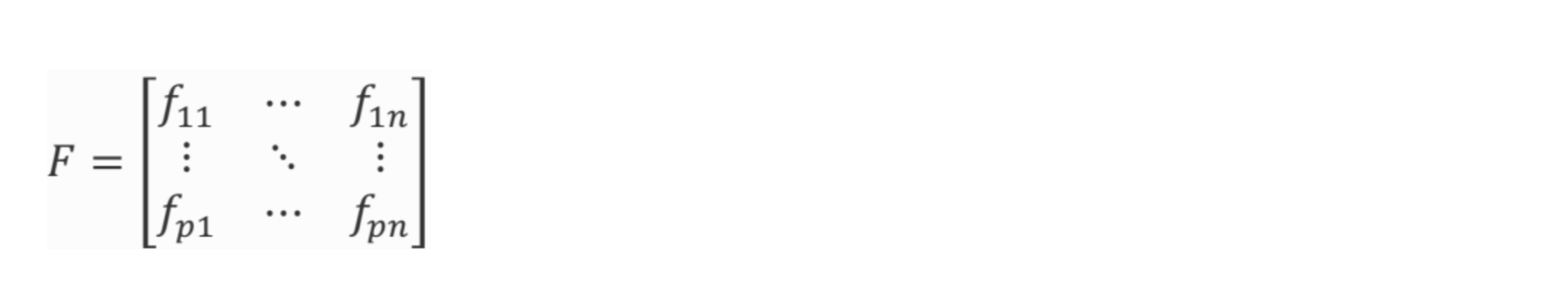
where the value of the field at discrete time $t_i$ and spatial grid point $s_j$ is denoted by $f_{ij}$ for i = 1, … , p and j = 1, … , n. I obtain the sample covariance matrix, B as

Since the EOF aims to find the uncorrelated linear combinations of different variables that explain maximum variance. This translates mathematically to find a unit length direction $\vec{u}$ such that $F\vec{u}$ has maximum variability. This can be expressed as

The above equation can be achieved by considering an eigenvalue problem $b_{ij}\vec{u} = \lambda^{2}\vec{u}$. Here, I decompose the data matrix F directly, using the Singular Value Decomposition approach (Golub & Van Loan 1996), as

where $A$ and $U$ are respectively $p \times r$ and $r \times n$ unitary matrix ($U^TU = A^TA = I_r$) and $r \leq \min(n, p)$ is the rank of $F$. The diagonal matrix $\Lambda = \mathrm{Diag}(\lambda_1,\lambda_2,…,\lambda_r)$. The columns of A ($a_1, a_2,…,a_r$), and U ($u_1, u_2,…,u_r$) respectively are the EOFs and principal components (PCs) of the data matrix F. To improve the computation of above equation, it is advisable to take the $\min(p,n)$ as the first dimension of F. The EOFs, A are orthogonal and the PCs, U are uncorrelated. Hence, the Equation above yields the decomposition

Accounted variance

The principal components and the corresponding eigenvectors respectively represent the temporal and spatial part of the given input data matrix F. I arrange the eigenvectors in decreasing order of eigenvalues, such that the first PC represent the biggest contributor to the variance of the space-time field. It is conventional to write the accounted variance in percentage as

The spectrum of the covariance matrix B provides information on the distribution of power (or energy) as a function of scale, and on the separation (or degeneracy) of the EOF patterns (represented as modes). The high and low power respectively are most commonly associated with the low and high frequency variability. Hence, low frequency (and large scale) patterns tends to capture most of the observed variance in the system.

If two eigenvalues are degenerate (or indistinguishable within estimated uncertainties), then their corresponding EOF pattern can possibly mix and may not be particularly interesting.

Application on the GPS data of Taiwan (Kumar et al., 2020)

I constructed the space-time data matrix of the GPS residuals for the daily time samples for 10 years, and 47 selected stations. EOF retrieves the coherent spatio-temporal signals mathematically by solving for a series of eigenmodes of the covariance matrix expressed in standing oscillations in the form of the product of spatial pattern and time series for a given target region and selected timespan (Chao & Liau 2019; Chang & Chao 2014). I arranged the eigenmodes in decreasing order of (the positive) eigenvalues, such that the first eigenmode represents the biggest contributor to the variance (measured by the ratio of the eigenvalue for the given mode index to the sum of all eigenvalues) of the GPS residuals.

Here the first mode is for the CME, while the higher modes reflect secondary effects or local and short-period signals or noises not of interest here. The calculated eigenvalue spectrum of the EOF along with their standard errors (calculated using Monte Carlo simulations) shows that the first mode is nondegenerate and separated from the rest.

I normalize the spatial pattern for the first mode by dividing with the RMS value (given that it is near-uniform in space), whereas for the second mode by dividing with the standard deviation (given its fluctuation around 0). The corresponding time series, or principal components, are scaled by multiplying by the same normalization value, transferring the magnitude information of eigenvectors into the principal components, which hence has the same unit as the data (mm in our study).

MATLAB Function for EOF analysis

Consider citing Kumar et al., 2020, if you use the codes.

function [eigenValues, varpercent, eofMapPattern, eof_temp_coeff] = eof_n_optimizado_A(data)


Z=detrend(Matrix,'constant'); %removes the mean value from each column of the matrix

% the matrix dimensions: 
% n = number of temporal samples
% p = number of points with data
[n,p] = size(Z);

% If n>=p we estimate the EOF in the State Space Setting, i.e., using Z'*Z which is p x p.
% If n<p  we estimate the EOF in the Sample Space Setting, i.e., using Z*Z' which is n x n 
if n>=p
    
    %%%%%%%%%%%%%%%%%%%%%%%%%%%
    %%% State Space Setting %%%
    %%%%%%%%%%%%%%%%%%%%%%%%%%%
    
    % Covariance matrix
    R=Z'*Z;
    
    % We estimate the eigenvalues and eigenvectors of the covariance matrix.
    [eof_p,L]=eigs(R, eye(size(R)),10);       % The eigenvelues are in the diagonal of L
                            % and the associated eigenvectors are in the columns of eof_p

    eigenValues=diag(L);                    
    
    % We estimate the expansion coefficients (time series) associated to each EOF
    [a,b]=size(L);
    for i=1:a
        exp_coef(:,i)= Z * eof_p(:,i);
    end
    
elseif n<p
    
    %%%%%%%%%%%%%%%%%%%%%%%%%%%%
    %%% Sample Space Setting %%%
    %%%%%%%%%%%%%%%%%%%%%%%%%%%%
    fprintf('Sample space setting\n');
    % Scatter matrix
    R=Z*Z';
    
    % We estimate the eigenvalues and eigenvectors of the scatter matrix.
    [eof_p_f,L]=eigs(R, eye(size(R)),10);     % The eigenvelues are in the diagonal of M
                            % and the associated eigenvectors are in the columns of eof_p_f
                            
    eigenValues=diag(L);
    
    % We estimate the expansion coefficients (time series) associated to each EOF
    [a,b]=size(L);
    for i=1:a
        exp_coef_b(:,i)= Z' * eof_p_f(:,i);
    end
    
    % We transform the EOF and their associated expansion coefficient (time series) in the Sample 
    % space setting to those in the State space setting
    
    %Expansion coefficients
    for i=1:a
        eof_p(:,i)= exp_coef_b(:,i) / sqrt(eigenValues(i));
    end
    
    %Expansion coefficients
    for i=1:a
        exp_coef(:,i)= sqrt(eigenValues(i)) * eof_p_f(:,i);
    end
    
end


% We estimate the percentage of variance explained by each EOF/eigenvector
varpercent = ( diag(L)/trace(L) )*100;

%We normalized the EOF
[a_1,b_1]=size(eof_p);
[a_11,b_11]=size(exp_coef);
eofMapPattern=eof_p;
eof_temp_coeff=exp_coef;

for i=1:b_1
    
    eofMapPattern(:,i) = eof_p(:,i)./ rms(eof_p(:,i));
    eof_temp_coeff(:,i) = exp_coef(:,i).* rms(eof_p(:,i));

%     using standard deviation
%     eofMapPattern(:,i) = eof_p(:,i)./ std(exp_coef(:,i));
%     eof_temp_coeff(:,i) = exp_coef(:,i) .* std(exp_coef(:,i));

    
end

Recap

• EOF = PCA on a space–time field. Arrange data as time × location, and decompose it into modes, each a spatial pattern (EOF) × a temporal series (PC).
• SVD does the work. $F = A\Lambda U^{T}$ (or eigen-decomposition of the covariance $F^{T}F$) yields orthogonal EOFs and uncorrelated PCs in one shot.
• Rank by variance. Eigenvalues order the modes; the largest capture the dominant coherent signal (e.g. the common-mode error in the GPS study), and you keep only the first few.
• Mind degeneracy. Nearly-equal eigenvalues mean the modes can mix and shouldn’t be over-interpreted individually.

Where to go next

• NumPy linalg.svd (the Python equivalent of the MATLAB code): numpy.org/doc/stable/reference/generated/numpy.linalg.svd.html
• The eofs package (EOF analysis with weighting/xarray support): ajdawson.github.io/eofs
• The GPS application paper (open access): What Causes the Common-Mode Error in Array GPS Displacement Fields

References

1. Fukuoka, A. (1951). A study on 10-day forecast (A synthetic report). Geophysical Magazine, 22(3), 177–208. CiNii record
2. Lorenz, E. N. (1956). Empirical Orthogonal Functions and Statistical Weather Prediction. Scientific Report No. 1, Statistical Forecasting Project, Department of Meteorology, MIT.
3. Application of the Karhunen–Loève expansion to feature selection and ordering — Fukunaga, K., & Koontz, W. L. G., 1970, IEEE Transactions on Computers, C-19(4), 311–318.
4. Golub, G. H., & Van Loan, C. F. (1996). Matrix Computations (3rd ed.). Johns Hopkins University Press.
5. Gravity Changes Due to Large Earthquakes Detected in GRACE Satellite Data via Empirical Orthogonal Function Analysis — Chao, B. F., & Liau, J. R., 2019, Journal of Geophysical Research: Solid Earth, 124(3), 3024–3035.
6. Analysis of coseismic deformation using EOF method on dense, continuous GPS data in Taiwan — Chang, E. T. Y., & Chao, B. F., 2014, Tectonophysics, 637, 106–115.
7. What Causes the Common-Mode Error in Array GPS Displacement Fields: Case Study for Taiwan in Relation to Atmospheric Mass Loading — Kumar, U., Chao, B. F., & Chang, E. T.-Y., 2020, Earth and Space Science, 7(9), e2020EA001159.

References

- Fukuoka, A. (1951). The Central Meteorological Observatory, A study on 10-day forecast (A synthetic report). Geophysical Magazine, 22(3), 177–208. Retrieved from http://ci.nii.ac.jp/naid/40018672317/en/