Exploratory Factor Analysis (codes included)

Data with large number of measured variables have the possibility of having some variables to “overlap” due to its inherent dependency. Factor Analysis (FA) is an exploratory data analysis method used to search influential underlying factors or latent variables from a set of observed variables. It is a method for investigating whether a number of variables of interest Y1, Y2,…, Yl, are linearly related to a smaller number of unobservable factors F1, F2,…, Fk.

Data and Methods

We have data for the Individuals entering web-based personality assessment tests for 25 personalities. These 25 variables (A1, A2, …, O5) can be organized by five putative factors: Agreeableness, Conscientiousness, Extraversion, Neuroticism, and Openness.

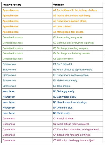
The data for each 25 variables were collected on a 6 point response scale – 1 Very Inaccurate; 2 Moderately Inaccurate; 3 Slightly Inaccurate; 4 Slightly Accurate; 5 Moderately Accurate; 6 Very Accurate.

# Import required libraries
import pandas as pd
from sklearn.datasets import load_iris
from factor_analyzer import FactorAnalyzer
import matplotlib.pyplot as plt
from matplotlib import style
import matplotlib
from factor_analyzer.factor_analyzer import calculate_bartlett_sphericity
from factor_analyzer.factor_analyzer import calculate_kmo


matplotlib.rcParams['figure.figsize'] = (10.0, 6.0)

style.use('ggplot')

df= pd.read_csv("bfi.csv")
df.drop(['Unnamed: 0','gender', 'education', 'age'],axis=1,inplace=True)
# Dropping missing values rows
df.dropna(inplace=True)

The Factor Analysis Model

Factor analysis can statistically explain the variance among the observed variable and condense a set of the observed variable into the unobserved variable called factors. Observed variables are modeled as a linear combination of factors and error terms. Each factor explains a particular amount of variance in the observed variables and can help in data interpretations by reducing the number of variables.

What is the Factor?

The factor is a latent variable that describes the association among the number of observed variables. The maximum number of factors is equal to the number of observed variables. Every factor explains a certain variance in observed variables. The factors with the lowest amount of variance were dropped (source).

What are factor loadings?

The factor loading is a matrix which shows the relationship of each variable to the underlying factor. It shows the correlation coefficient for the observed variable and factor. It shows the variance explained by the observed variables (source).

Adequacy Test

Before we perform factor analysis, we need to evaluate the “factorability” of our dataset. Factorability means “can we find the factors in the dataset?”. There are two methods to check the factorability:

1. Bartlett’s Test
2. Kaiser-Meyer-Olkin Test

Bartlett’s Test

Bartlett’s test of sphericity checks whether or not the observed variables intercorrelate at all using the observed correlation matrix against the identity matrix. If the test found statistically insignificant, we should not employ a factor analysis.

from factor_analyzer.factor_analyzer import calculate_bartlett_sphericity
chi_square_value,p_value=calculate_bartlett_sphericity(df)
chi_square_value, p_value

Kaiser-Meyer-Olkin (KMO) Test

It is a statistic that indicates the proportion of variance in our variables that might be caused by underlying factors. High values (close to 1.0) generally indicate that a factor analysis may be useful with our data. If the value is less than 0.50, the results of the factor analysis probably won’t be very useful.

from factor_analyzer.factor_analyzer import calculate_kmo
kmo_all,kmo_model=calculate_kmo(df)

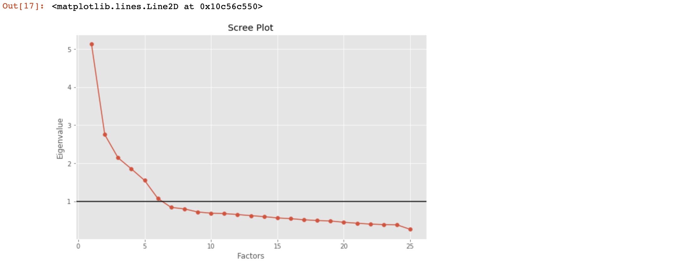
Choosing the Number of Factors

The eigenvalue is a good criterion for determining the number of factors. Generally, an eigenvalue greater than 1 will be considered as selection criteria for the feature.

# Create factor analysis object and perform factor analysis
fa = FactorAnalyzer()
fa.analyze(df, 25, rotation=None)
# Check Eigenvalues
ev, v = fa.get_eigenvalues()
ev

factor_analyzer’s API changed — update these calls. This post uses the old (pre-0.3) interface: FactorAnalyzer() followed by fa.analyze(df, n, rotation=...) and the fa.loadings attribute. In the current package (0.5.x) the analyze() method is gone — you set the options in the constructor and call fit instead, and the loadings attribute now ends in an underscore:

# modern factor_analyzer (>= 0.3)
fa = FactorAnalyzer(n_factors=25, rotation=None)
fa.fit(df)
ev, v = fa.get_eigenvalues()        # unchanged
# ... then, e.g.
fa = FactorAnalyzer(n_factors=6, rotation="varimax")
fa.fit(df)
fa.loadings_                         # note the trailing underscore

get_eigenvalues(), get_factor_variance(), calculate_bartlett_sphericity, and calculate_kmo all still work as shown. The logic and results are identical — only the call style moved.

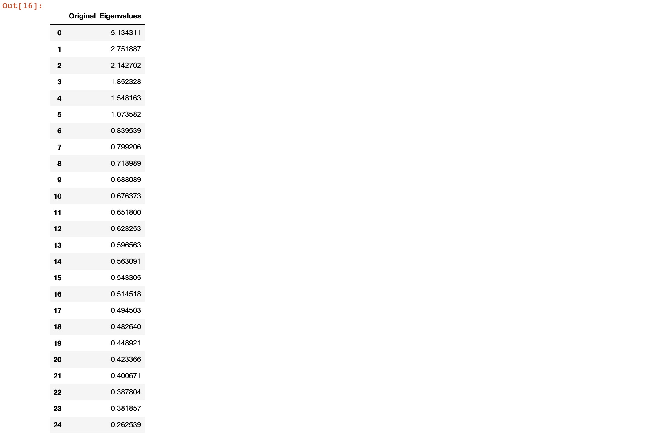
Here, we can see only for 6-factors eigenvalues are greater than one. It means we need to choose only 6 factors (or unobserved variables).

# Create scree plot using matplotlib
plt.scatter(range(1,df.shape[1]+1),ev.values)
plt.plot(range(1,df.shape[1]+1),ev.values)
plt.title('Scree Plot')
plt.xlabel('Factors')
plt.ylabel('Eigenvalue')
plt.axhline(y=1,c='k')

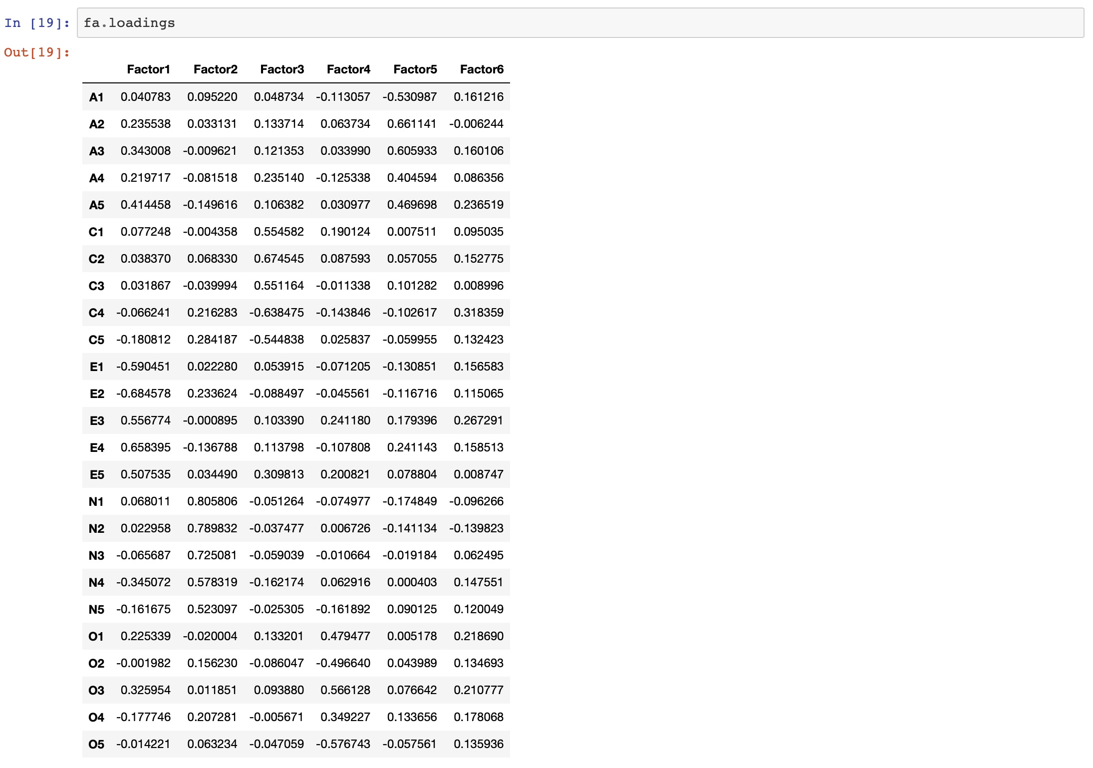
Performing Factor Analysis

# Create factor analysis object and perform factor analysis
fa = FactorAnalyzer()
fa.analyze(df, 6, rotation="varimax")
fa.loadings

import numpy as np
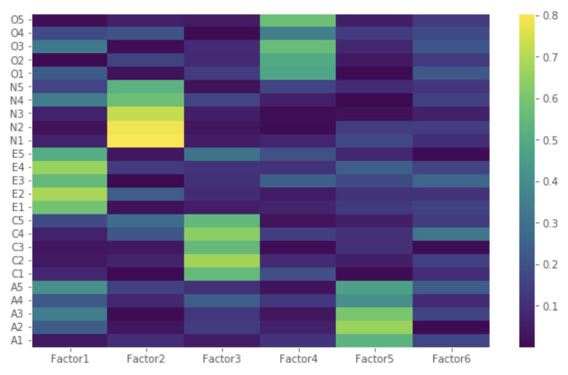
Z=np.abs(fa.loadings)
fig, ax = plt.subplots()
c = ax.pcolor(Z)
fig.colorbar(c, ax=ax)
ax.set_yticks(np.arange(fa.loadings.shape[0])+0.5, minor=False)
ax.set_xticks(np.arange(fa.loadings.shape[1])+0.5, minor=False)
ax.set_yticklabels(fa.loadings.index.values)
ax.set_xticklabels(fa.loadings.columns.values)
plt.show()

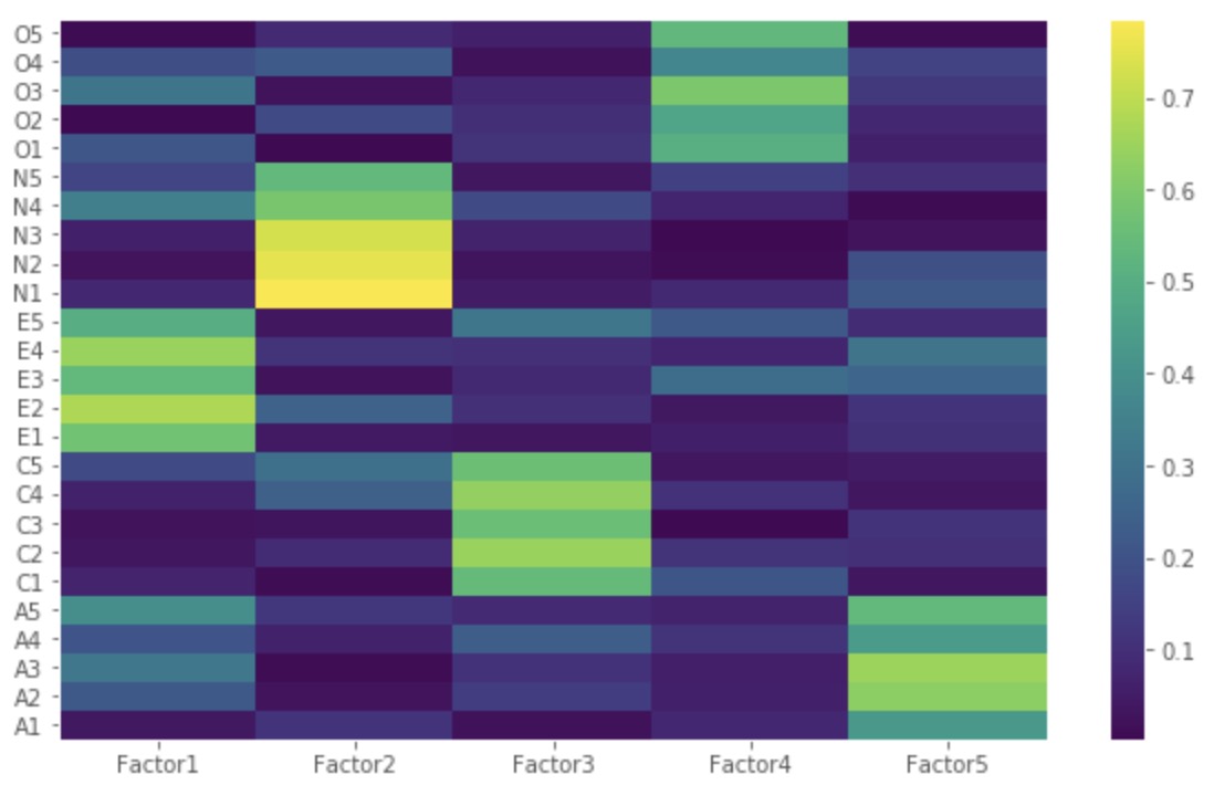
• Factor 1 has high factor loadings for E1,E2,E3,E4, and E5 (Extraversion)

• Factor 2 has high factor loadings for N1, N2, N3, N4, and N5 (Neuroticism)

• Factor 3 has high factor loadings for C1,C2,C3,C4, and C5 (Conscientiousness)

• Factor 4 has high factor loadings for O1,O2,O3,O4, and O5 (Opennness)

• Factor 5 has high factor loadings for A1,A2,A3,A4, and A5 (Agreeableness)

• Factor 6 has none of the high loadings for any variable and is not easily interpretable. Its good if we take only five factors.

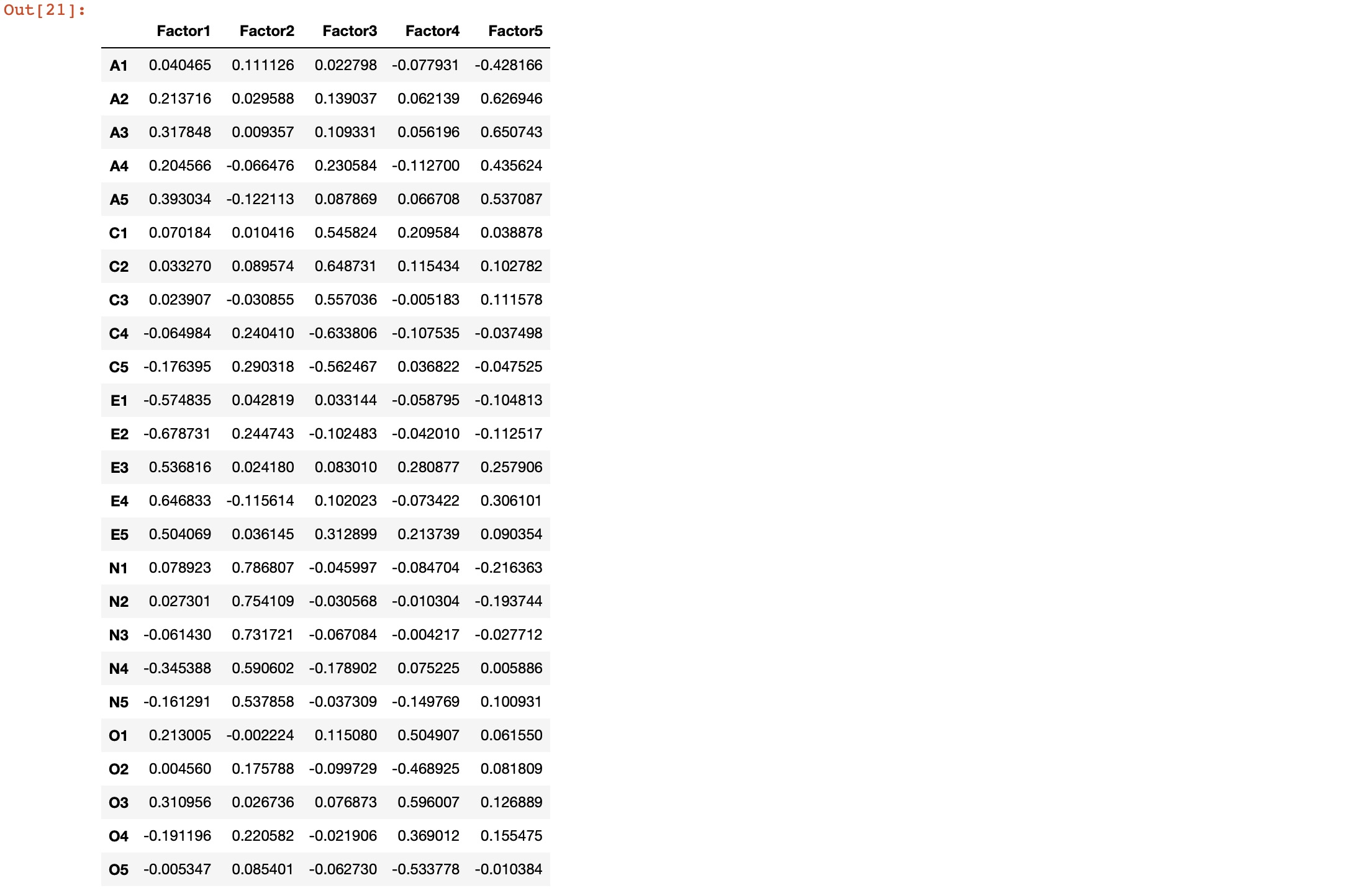
Let’s perform factor analysis for 5 factors.

# Create factor analysis object and perform factor analysis using 5 factors
fa = FactorAnalyzer()
fa.analyze(df, 5, rotation="varimax")
fa.loadings

Z=np.abs(fa.loadings)
fig, ax = plt.subplots()
c = ax.pcolor(Z)
fig.colorbar(c, ax=ax)
ax.set_yticks(np.arange(fa.loadings.shape[0])+0.5, minor=False)
ax.set_xticks(np.arange(fa.loadings.shape[1])+0.5, minor=False)
ax.set_yticklabels(fa.loadings.index.values)
ax.set_xticklabels(fa.loadings.columns.values)
plt.show()

Let us now obtain the variance for each factor:

# Get variance of each factors
fa.get_factor_variance()

The total cumulative variance explained by the 5 factors is 100*0.423619 = ~42%.

Recap

• Factor analysis models each observed variable as a weighted sum of a few latent factors (the loadings) plus unique noise — it explains the correlations among many variables with fewer hidden ones.
• Check factorability first: Bartlett’s test should be significant (variables do intercorrelate) and the KMO measure should be well above 0.5.
• Choose the number of factors from the eigenvalues — keep those > 1 (Kaiser criterion) or read the elbow of the scree plot.
• Rotate (e.g. varimax) so each factor loads cleanly on one interpretable group; here five factors recovered the Big Five personality traits, while the sixth was uninterpretable and dropped.
• EFA is a latent-variable model (factors → variables); PCA is a variance-maximizing transform (variables → components) — related tools, opposite direction of explanation.

Where to go next

• Principal Component Analysis to decompose signal dimensionality — the variance-maximizing cousin of factor analysis.
• Empirical Orthogonal Function analysis of geospatial data — PCA/EOF applied to spatial fields.
• How to start using pandas for Earth data analysis — the dataframe handling used to load and clean the data here.

References:

1. DataCamp — Introduction to Factor Analysis in Python
2. P. Tryfos — Factor Analysis (York University)
3. MATLAB — Factor Analysis