Numerically solving initial value problems using the Runge-Kutta method
In the last post, we discussed about the Euler method to solve the initial value problems. Euler method is simplistic approach for such problems but it comes with large inaccuracy. We will now discuss the Runge-Kutta method for solving such problems.
Key idea — sample the slope several times per step, then average. Euler takes one step using only the slope at the left end of the interval, so it drifts. Runge-Kutta instead probes the slope at several points inside each step — the start, the midpoint (twice), and the end — and advances using a weighted average of them. More slope samples per step means the error shrinks dramatically: RK4 accumulates error like $O(\Delta t^4)$ versus Euler’s $O(\Delta t)$, for the same step size.
Runge-Kutta methods
Runge-Kutta methods are used to solve ordinary differential equations (ODEs) with a better approximation than the Euler method. For the Euler method, we ended with an iterative scheme:
\[\vec{y}_{n+1} = \vec{y}_n + \Delta t . \phi\]where the function $\phi$ is chosen to reduce the error over a single time-step, $\Delta t$. For the Runge-Kutta methods, we no longer have to constrain the function $\phi$ to make use of the derivative at the left end point of the computational step. We also compute the derivative at the midpoint and at the right end of the time-step to possibly improve the accuracy.
In theory, the Euler method is the first-order Runge Kutta method. Heun’s, midpoint, and Ralston method is the second-order Runge Kutta method that uses two derivatives.
Third-order Runge-Kutta
For an ODE:
\[\frac{d\vec{y}}{dt} = f(t,\vec{y})\]where, at $t=t_0$, $\vec{y}(0) = \vec{y}_0$. In this post, we assume $h = \Delta t$. The iterative scheme for the third-order Runge Kutta is:
\[\vec{y}_{n+1} = \vec{y}_n + (1/6)h . (k_1 + 4 k_2 + k_3)\]where,
\[k_1 = f(t,\vec{y})\] \[k_2 = f(t+h/2,\vec{y}+(h/2).k_1)\] \[k_3 = f(t+h/2,\vec{y}+h.(-k_1 + 2k_2))\]Fourth-order Runge-Kutta
The most popular general stepping scheme used in practice is the fourth-order Runge Kutta method. In this case, the Taylor series local truncation error is pushed to $O(\Delta t^5)$, and the total cumulative error becomes $O(\Delta t^4)$. Hence, the name “fourth-order”.
For an ODE:
\[\frac{d\vec{y}}{dt} = f(t,\vec{y})\]where, at $t=t_0$, $\vec{y}(0) = \vec{y}_0$. The iterative scheme for the fourth-order Runge Kutta is:
\[\vec{y}_{n+1} = \vec{y}_n + h . T_4(t,\vec{y},h)\]Here, $T_4$ is
\[T_4 = \frac{1}{6}(k_1 + 2k_2 + 2k_3 + k_4)\] \[k_1 = f(t,\vec{y})\] \[k_2 = f(t+h/2,\vec{y}+(h/2).k_1)\] \[k_3 = f(t+h/2,\vec{y}+(h/2).k_2)\] \[k_4 = f(t+h,\vec{y}+h.k_3)\]Quick check: Why do $k_2$ and $k_3$ carry a weight of 2 in the RK4 update, while $k_1$ and $k_4$ carry a weight of 1?
Example problem
\[\frac{dy}{dt} = sin(t)^2 * y\]where, the initial conditions are $t(0)=1$, and $y(0)=2$. We can use the step size of $h=0.5$.
Here, the general solution of this differential equation is:
\[y = 2 e^{0.5*(t-sin(t)cos(t))} + c\]Solving Example problem using Python
We can solve the ODE using the third and fourth-order Runge-Kutta method and compare the estimation with the analytical solution.
import numpy as np
import matplotlib.pyplot as plt
plt.style.use('seaborn')

# define equations

def dydt(t, y): return np.sin(t)**2*y
def f(t): return 2*np.exp(0.5*(t-np.sin(t)*np.cos(t)))


def RK3(t, y, h):
    # compute approximations
    k_1 = dydt(t, y)
    k_2 = dydt(t+h/2, y+(h/2)*k_1)
    k_3 = dydt(t+h/2, y+h*(-k_1 + 2*k_2))

    # calculate new y estimate
    y = y + h * (1/6) * (k_1 + 4 * k_2 + k_3)
    return y


def RK4(t, y, h):
    # compute approximations
    k_1 = dydt(t, y)
    k_2 = dydt(t+h/2, y+(h/2)*k_1)
    k_3 = dydt(t+h/2, y+(h/2)*k_2)
    k_4 = dydt(t+h, y+h*k_3)

    # calculate new y estimate
    y = y + h * (1/6)*(k_1 + 2*k_2 + 2*k_3 + k_4)
    return y


# Initialization
ti = 0
tf = 5
h = 0.5
n = int((tf-ti)/h)
t = 0
y = 2
y_rk3 = 2

print("t \t\t yRK3 \t\t yRK4 \t\t f(t)")
print(f"{t:.1f} \t\t {y_rk3:4f} \t\t {y:4f} \t\t {f(t):.4f}")

t_plot = []
y_RK3 = []
y_RK4 = []
y_analytical = []


##
for i in range(1, n+1):
    t_plot.append(t)
    y_RK4.append(y)
    y_RK3.append(y_rk3)
    y_analytical.append(f(t))

    # calculate new y estimate
    y = RK4(t, y, h)
    y_rk3 = RK3(t, y_rk3, h)

    t += h
    print(f"{t:.1f} \t\t {y_rk3:4f} \t\t {y:4f} \t\t {f(t):.4f}")


t_plot.append(t)
y_RK3.append(y_rk3)
y_RK4.append(y)
y_analytical.append(f(t))


# Visualization
fig, (ax, ax2) = plt.subplots(2, 1)
ax.plot(t_plot, y_analytical, 'ro', label='Analytical solution')
ax.plot(t_plot, y_RK4, '.b', label='Fourth-order Runge-Kutta estimate')
ax.plot(t_plot, y_RK3, '.g', label='Third-order Runge-Kutta estimate')
ax.set_ylabel("y", fontsize=18)
ax.legend()

ax2.plot(t_plot, np.abs(np.array(y_analytical) -
                        np.array(y_RK4)), '.-b', label='Fourth-order Runge-Kutta')
ax2.plot(t_plot, np.abs(np.array(y_analytical) -
                        np.array(y_RK3)), '.-g', label='Third-order Runge-Kutta')
ax2.set_ylabel("Abs Error", fontsize=18)
ax2.legend()
ax2.set_xlabel("t", fontsize=18)
plt.savefig('runge_kutta_analytical.png', dpi=300, bbox_inches='tight')
t                yRK3                     yRK4                    f(t)
0.0              2.000000                2.000000                2.0000
0.5              2.051632                2.080616                2.0809
1.0              2.536277                2.626551                2.6269
1.5              3.906789                4.086093                4.0872
2.0              6.344784                6.566018                6.5689
2.5              8.748588                8.867524                8.8718
3.0              9.576568                9.606408                9.6119
3.5              9.639375                9.759067                9.7659
4.0              11.154816               11.531199               11.5399
4.5              16.305226               17.103444               17.1178
5.0              26.714744               27.886259               27.9147
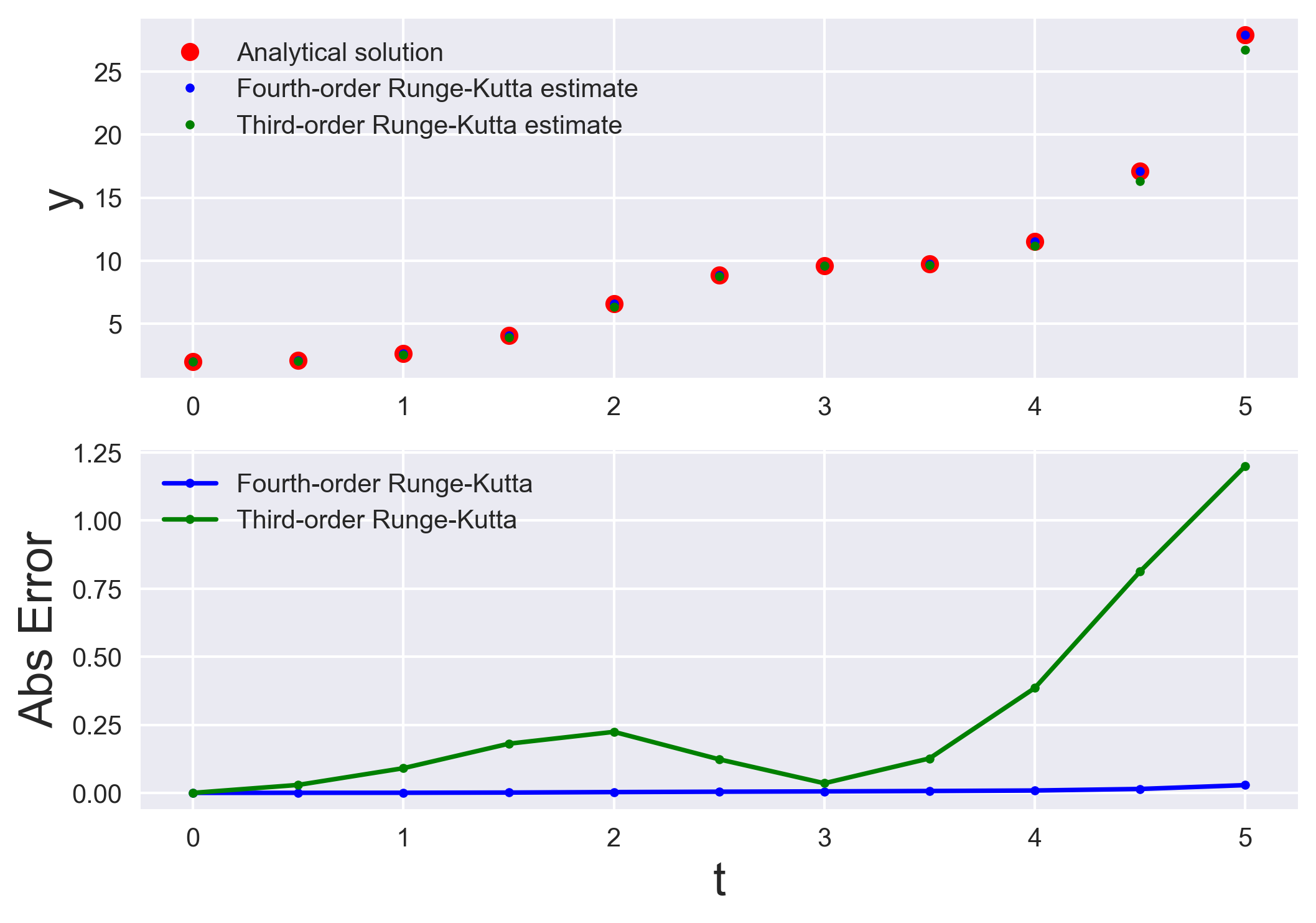
Read the table as a race against the truth. The f(t) column is the exact answer. Notice the fourth-order column tracks it to ~3 decimal places, while the third-order column drifts noticeably by t = 5 (26.71 vs the true 27.91). The lower error-plot in the figure makes the gap explicit — same step size, but each extra order of the method buys a big accuracy jump.
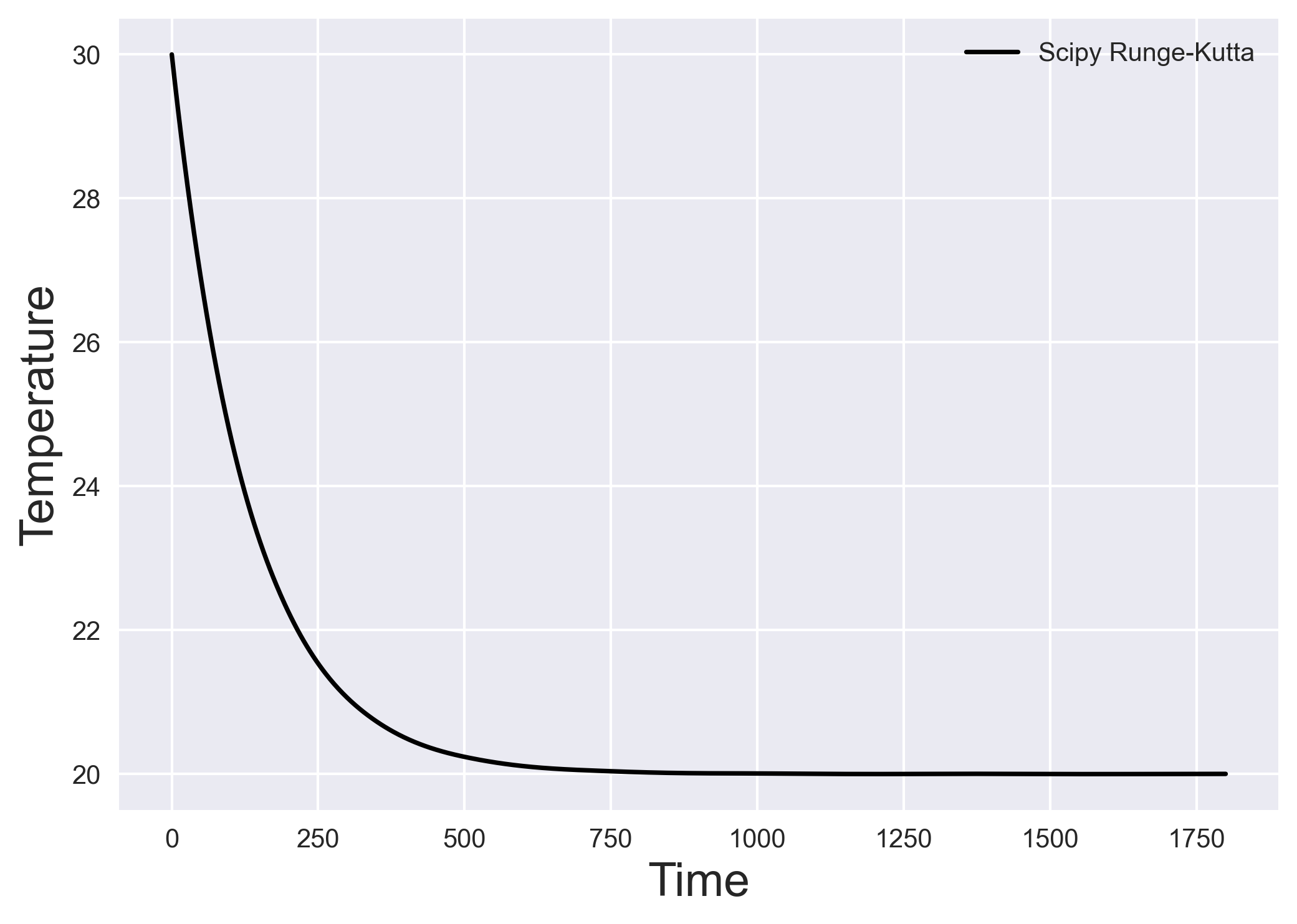
Heat transfer problem using fourth-order Runge Kutta
We can solve the heat transfer problem from the previous post using the scipy’s scipy.integrate.solve_ivp function. It uses explicit Runge-Kutta method of order 5. The error is controlled assuming accuracy of the fourth-order method, but steps are taken using the fifth-order accurate formula (local extrapolation is done).
For the heat transfer problem, We find the temperature profile of an object in contact with a constant temperature surface through a thermal conductance.
\[\frac{dT}{dt} = -\frac{k}{c} (T-T_f)\]where $T_f$ is the constant temperature of the surface, $k$ is the thermal conductance, $c$ is the specific heat of the object, and $T$ is the variable temperature of the object. Here, we know the temperature of the object at $t=0$.
\[T(0) = 30\]import numpy as np
import matplotlib.pyplot as plt
from scipy.integrate import solve_ivp
plt.style.use('seaborn')
# the governing equation
def heat_equations(t, T):
k = 0.075
C = 10
T_f = 20
return -k * (T - T_f) / C
# Time steps
teval = np.linspace(0, 1800, 1000)
# ivp solver: Runge-Kutta
sol = solve_ivp(heat_equations, (teval[0], teval[-1]), (30,), t_eval=teval)
fig, ax = plt.subplots()
ax.plot(sol.t, sol.y[0, :], "-k", ms=3, label='Scipy Runge-Kutta')
ax.set_ylabel("Temperature", fontsize=18)
ax.set_xlabel("Time", fontsize=18)
plt.legend()
plt.savefig('runge_kutta_heat_transfer_sol.png', dpi=300, bbox_inches='tight')
Two small modernizations. scipy.integrate.solve_ivp (used here) is the recommended ODE interface today — its default method='RK45' is exactly the adaptive fifth-order Runge–Kutta described above, and it superseded the older odeint. Also, plt.style.use('seaborn') was removed in Matplotlib 3.8; use plt.style.use('seaborn-v0_8') on a current install. The numerical code itself is unchanged.
Recap
- RK beats Euler by sampling more slopes. Euler uses one left-endpoint slope; RK samples the interior and endpoint too, then averages.
- RK4 is the workhorse. Four slope evaluations ($k_1$…$k_4$), combined with weights 1-2-2-1, give $O(\Delta t^4)$ cumulative error — accurate enough for most problems.
- Order costs evaluations, buys accuracy. The example table shows RK4 hugging the analytical curve where RK3 visibly drifts, at the same step size.
- In practice, reach for
solve_ivp. SciPy’s adaptive RK45 handles step-size control for you and replaces hand-rolled loops for production work.
Where to go next
scipy.integrate.solve_ivpdocs: docs.scipy.org/doc/scipy/reference/generated/scipy.integrate.solve_ivp.html- Previous post — the Euler method: Numerically solving IVPs using the Euler method
- Where BVPs come in — the shooting method: Solving boundary value problems using the shooting method
References
- Kutz, J. N. (2013). Data-driven modeling & scientific computation: methods for complex systems & big data. Oxford University Press.
Disclaimer of liability
The information provided by the Earth Inversion is made available for educational purposes only.
Whilst we endeavor to keep the information up-to-date and correct. Earth Inversion makes no representations or warranties of any kind, express or implied about the completeness, accuracy, reliability, suitability or availability with respect to the website or the information, products, services or related graphics content on the website for any purpose.
UNDER NO CIRCUMSTANCE SHALL WE HAVE ANY LIABILITY TO YOU FOR ANY LOSS OR DAMAGE OF ANY KIND INCURRED AS A RESULT OF THE USE OF THE SITE OR RELIANCE ON ANY INFORMATION PROVIDED ON THE SITE. ANY RELIANCE YOU PLACED ON SUCH MATERIAL IS THEREFORE STRICTLY AT YOUR OWN RISK.
Leave a comment