Numerically solving initial value problems using the Euler method

For scientific competition in geosciences, our goal is to solve or nonlinear partial differential equations of elliptic, hyperbolic, parabolic, or mixed type. We will begin by understanding the basic concepts for computationally solving initial value problems for ordinary differential equations (ODE). We can further build upon it to solve more complicated partial differential equations.

Computationally, we are required to approach the calculus problems from our high school in a slightly different manner. Whereas we have learned to take a limit in order to define a derivative or integral, in the numerical approach, we take the derivative or integral of the governing equation and go backward to define it as a difference. It will become more apparent later when we solve the problems.

Initial Value Problems

We begin by considering a system of differential equations of the form:

where $\vec{y}$ represents the solution vector of interest, and the general function $f$ models the specific system of interest. These form of equations explain the dynamical evolution of a given system. In many cases, we know the initial conditions of such systems:

with $t \in [0,T]$.

Euler method

The most straightforward algorithm to solve this system of differential equations is known as the Euler method. The assumption is that over a time-span $\Delta t = t_{n+1} - t_n$, we can approximate the original differential equation by

From the above equation, we get

Thus, the Euler method gives an iterative scheme by which the future values of the solution can be determined. Graphically, the slope (derivative) of a function is responsible for generating each subsequent approximation of the solution $\vec{y}(t)$. It is important to note that the truncation error in the above equation is $O(\Delta t^2)$

Solving Example problem in Python

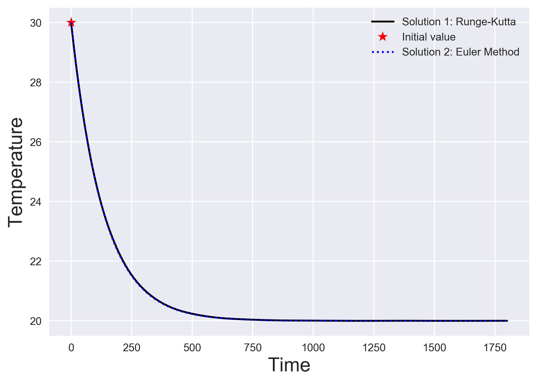
We will look into a simple heat transfer problem. We will find the temperature profile of an object in contact with a constant temperature surface through a thermal conductance. This problem is obtained from the youtube video Numerically Integrating Differential Equations in Excel and Python: Euler’s Method. The ODE of the system can be written as:

where $T_f$ is the constant temperature of the surface, $k$ is the thermal conductance, $c$ is the specific heat of the object, and $T$ is the variable temperature of the object. Here, we know the temperature of the object at $t=0$.

import numpy as np
import matplotlib.pyplot as plt
from scipy. integrate import solve_ivp
plt.style.use('seaborn')

# the governing equation


def heat_equations(t, T):
    k = 0.075
    C = 10
    T_f = 20
    return -k * (T - T_f) / C


# Time steps
teval = np.linspace(0, 1800, 1000)

# ivp solver: Runge-Kutta
sol = solve_ivp(heat_equations, (teval[0], teval[-1]), (30,), t_eval=teval)

fig, ax = plt.subplots()
ax.plot(sol.t, sol.y[0, :], "-k", ms=3, label='Solution 1: Runge-Kutta')


t = 0  # initial time
T = 30  # initial temperature

ax.plot([t], [T], "*r", ms=10, label='Initial value')

# Euler method: sol 2
time = [t]
temperature = [T]

delta_t = np.diff(teval)[0]  # 1.8018 for 1000 points

while t <= 1800:
    T += delta_t * heat_equations(t, T)
    t += delta_t
    time.append(t)
    temperature.append(T)

ax.plot(time, temperature, 'b:', ms=0.5, label='Solution 2: Euler Method')
ax.set_ylabel("Temperature", fontsize=18)
ax.set_xlabel("Time", fontsize=18)
plt.legend()
plt.savefig('euler_sol.png', dpi=300, bbox_inches='tight')

Conclusions

As you might have guessed, the Euler method has accuracy errors for complicated functions. This is the reason, Euler method is not used often in practice, but it is still a good starting point. In the future posts, we will look into the fourth-order Runge-Kutta method where the Taylor series local truncation error is pushed to $O(\Delta t^5)$

Recap

• An ODE gives you the slope; Euler walks it. $\vec{y}_{n+1} = \vec{y}_n + \Delta t\,f(t,\vec{y})$ is one tangent-line step, repeated across the interval.
• It’s first-order accurate. The local truncation error per step is $O(\Delta t^2)$; because the tangent ignores curvature, error accumulates — halving $\Delta t$ only roughly halves the global error.
• Great for intuition, weak for production. Euler is the clearest illustration of numerical integration, but real work uses higher-order schemes.
• Reach for the next method. The fourth-order Runge–Kutta samples the slope several times per step for far smaller error at the same step size.

Where to go next

• Next post — the Runge–Kutta method: Numerically solving IVPs using the Runge-Kutta method
• When both ends are fixed — the shooting method: Solving boundary value problems using the shooting method
• scipy.integrate.solve_ivp docs: docs.scipy.org/doc/scipy/reference/generated/scipy.integrate.solve_ivp.html

References

1. YouTube video: Numerically Integrating Differential Equations in Excel and Python: Euler’s Method
2. Kutz, J. N. (2013). Data-driven modeling & scientific computation: methods for complex systems & big data. Oxford University Press.