Time-Frequency Analysis in MATLAB (codes included)

Introduction

Signals can be any time-varying or space-varying quantity. Examples: speech, temperature readings, seismic data, stock price fluctuations.

A signal has one or more frequency components and can be viewed from two different standpoints: time-domain and frequency domain. In general, signals are recorded in the time-domain but analyzing signals in the frequency domain makes the task easier. For example, differential and convolution operations in the time domain become simple algebraic operations in the frequency domain.

Fourier Transform of a signal

We can go between the time-domain and frequency-domain by using a tool called Fourier transform.

Now to get comfortable with Fourier transform, let’s take an example in MATLAB:

clear; close all; clc

%%Creating dataset
fs=100;  %sampling frequency (samples/sec)
t=0:1/fs:1.5-1/fs;%time
f1=10; %frequency1
f2=20; %frequency2
f3=30; %frequency3

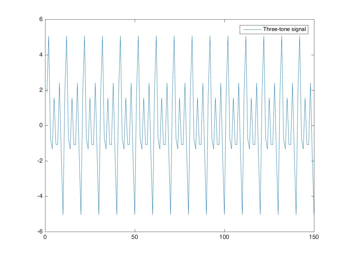
x=1*sin(2*pi*f1*t+0.3)+2*sin(2*pi*f2*t+0.2)+3*sin(2*pi*f3*t+0.4);

We represent the signal by the variable $x$. It is the summation of three sinusoidal signals with different amplitude, frequency, and phase shift. We plot the signal first.

%%Visualizing data
figure(1)
plot(x)
legend('Two-tone signal')
saveas(gcf,'signal_plot.jpg')

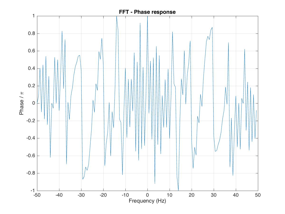
We then do the Fourier transform of the signal to obtain its magnitude and phase spectrum.

%%Fourier transform of the data
X=fft(x);
X_mag=abs(fftshift(X)); %magnitude
X_phase=angle(fftshift(X)); %phase

%%Frequency bins
N=length(x);
Fbins=(-N/2:N/2-1)/N*fs;


%%Magnitude response
figure(2);
plot(Fbins,X_mag)
xlabel('Frequency(Hz)')
ylabel('Magnitude')
title('FFT - Magnitude response')
grid on
saveas(gcf,'fft_mag_response.jpg')

%%Phase response
figure(3);
plot(Fbins,X_phase/pi)
xlabel 'Frequency (Hz)'
ylabel 'Phase / \pi'
title('FFT - Phase response')
grid on
saveas(gcf,'fft_phase_response.jpg')

Power spectrum estimation using the Welch’s method

Now we compute the power spectrum using the Welch’s method. We can use the function “pwelch” in Matlab to obtain the desired result.

pwelch(x,[],[],[],fs) %one-sided power spectral density
saveas(gcf,'power_spectral_plot.jpg')

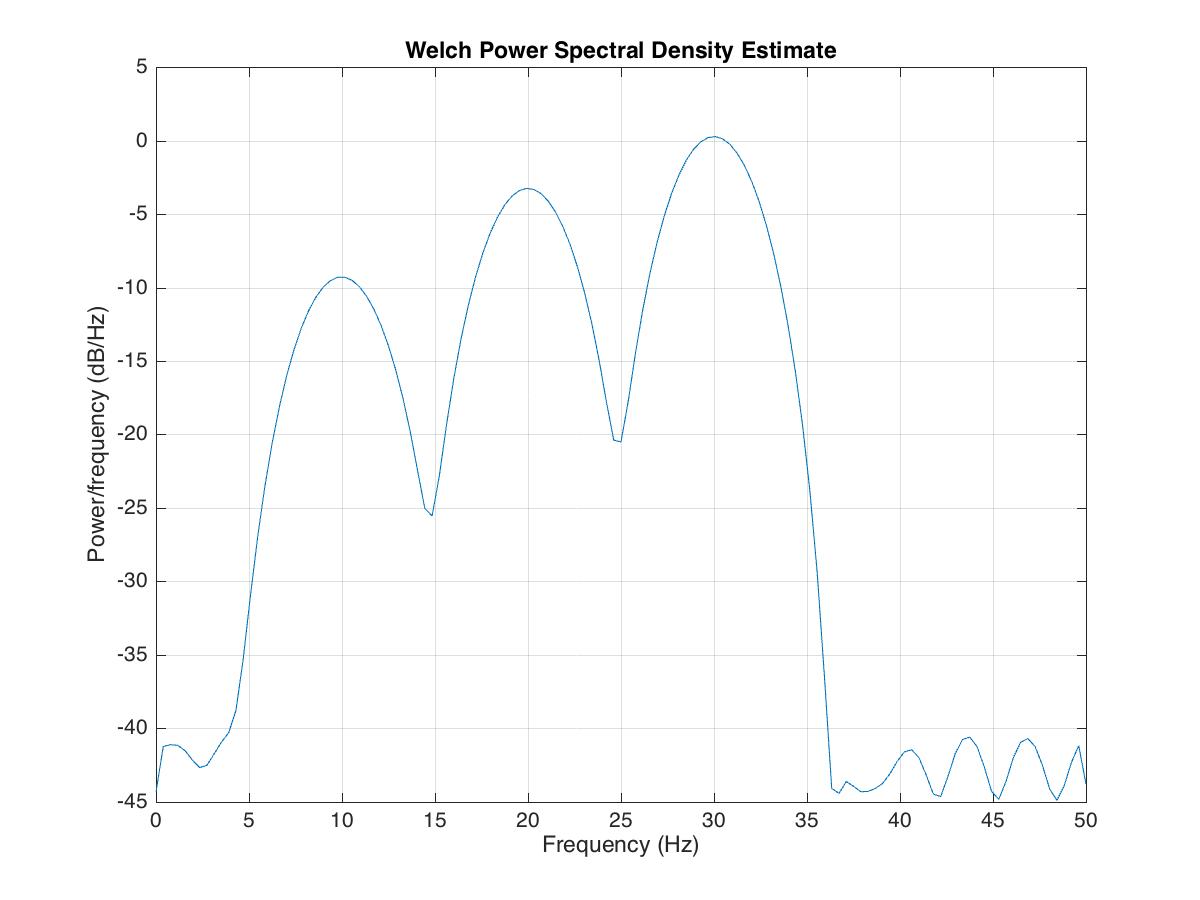
Pwelch is a spectrum estimator. It computes an averaged squared magnitude of the Fourier transform of a signal. In short, it computes a set of smaller FFTs (using sliding windows), computes the magnitude square of each, and averages them.

By default, $x$ is divided into the longest possible segments to obtain as close to but not exceed eight segments with 50% overlap. Each segment is windowed with a Hamming window. The modified periodograms are averaged to obtain the PSD estimate. If you cannot divide the length of $x$ precisely into an integer number of segments with 50% overlap, $x$ is truncated accordingly.

Note the peak at 10, 20, and 30 Hz. Also, note the display default for Pwelch is in dB (logarithmic).

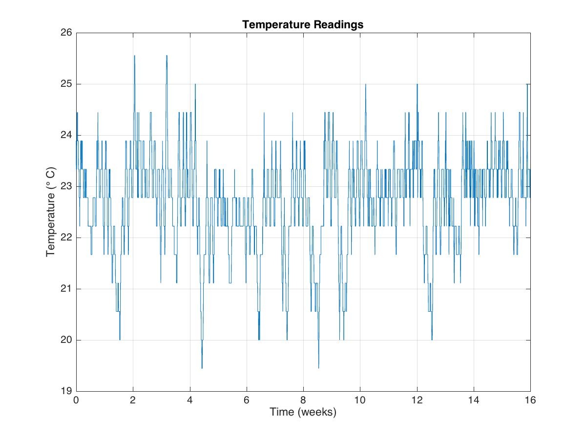
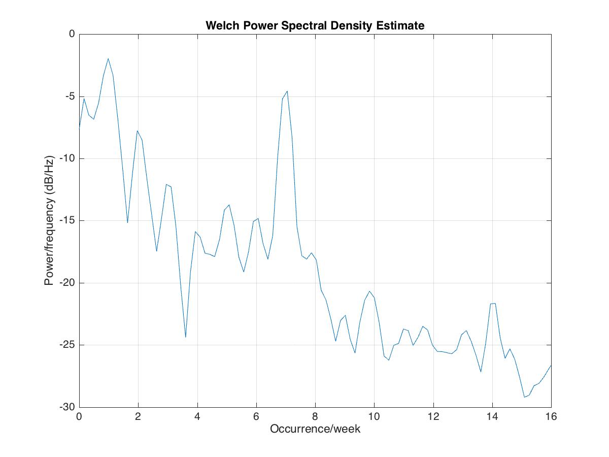
Let us inspect another data using the “pwelch” function of Matlab.

clear; close all; clc

load officetemp1; %16 weeks 2 samples/hr

%%Visualizing data
figure(1);
plot(t,tempC)
ylabel(sprintf('Temperature (%c C)', char(176)))
xlabel('Time (weeks)')
title('Temperature Readings')
grid on
saveas(gcf,'tempReadings.jpg')

tempnorm=tempC-mean(tempC); %temperature residual

fs=2*24*7; %2 samples per hour

figure(2);
pwelch(tempnorm,[],[],[],fs);
axis([0 16 -30 0])
xlabel('Occurrence/week')
saveas(gcf,'power_spectral_tempReadings.jpg')

Resolving two close frequency components using “pwelch”

Let’s first plot the data (having the frequency components at 500 and 550 Hz) using the default parameters of the “pwelch” function:

clear; close all; clc
load winLen;

%%

pwelch(s,[],[],[],Fs);
title('pwelch with default input- f1: 500Hz, f2: 550Hz')
set(gca,'YLim',[-120,0])
set(gca,'XLim',[0,5])

saveas(gcf,'pwelchDefaultPlot.jpg')

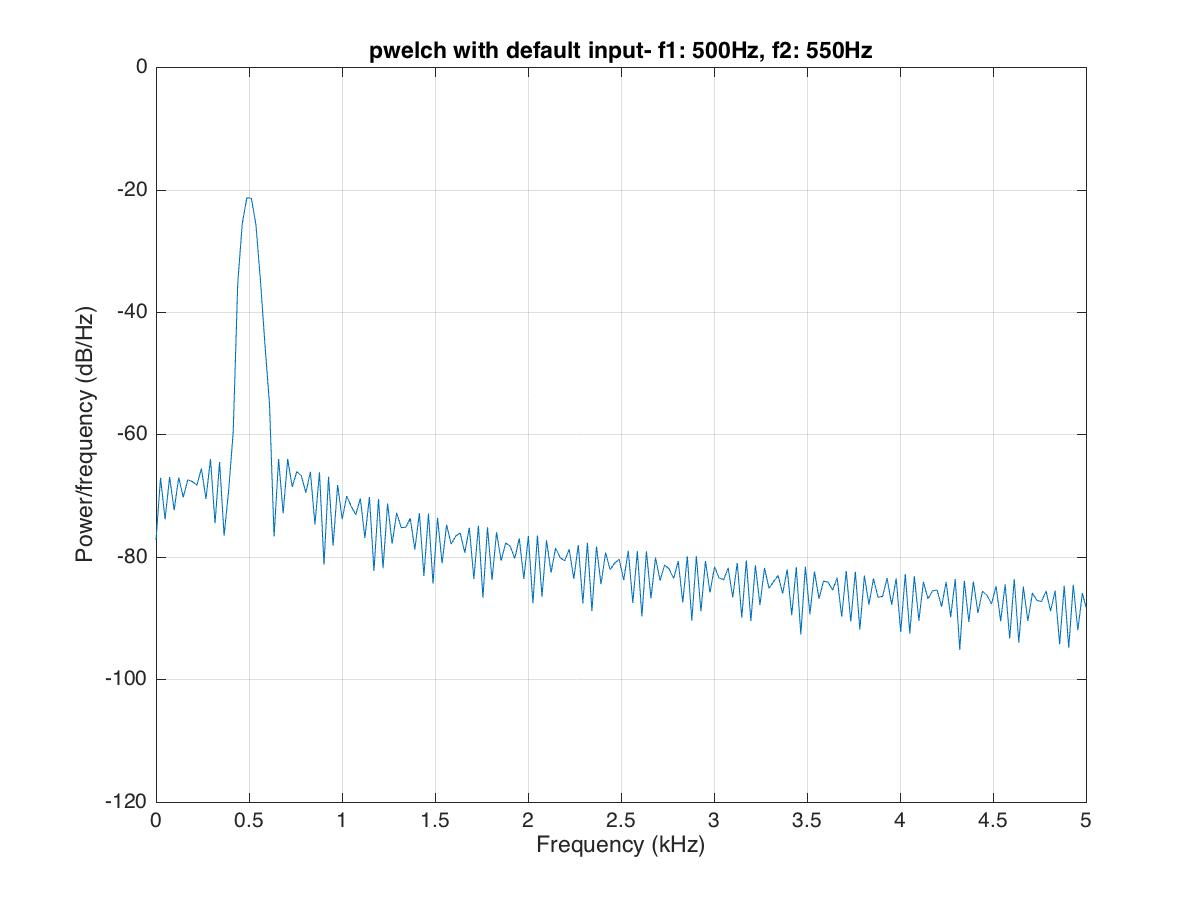
Here, we can see that the frequency component at 500Hz can be resolved, but the frequency component at 550 Hz is barely visible.

One can obtain better frequency resolution by increasing the window size:

figure;
filename = 'pwelchWindowAnalysis.gif';
for len=500:300:N
  pwelch(s,len,[],len,Fs);
  title(sprintf('Hamming Window size: %d',len))
  set(gca,'YLim',[-120,0])
  set(gca,'XLim',[0,1])
  drawnow;
  frame = getframe(1);
   im = frame2im(frame);
   [imind,cm] = rgb2ind(im,256);
   if len == 500;
     imwrite(imind,cm,filename,'gif', 'Loopcount',inf);
   else
     imwrite(imind,cm,filename,'gif','WriteMode','append');
   end
end

Here, we can see that by increasing the window width, we can resolve the two components. By increasing the window width, we lose the temporal resolution, but at the same time, we gain the spectral resolution.

Resolving the frequency component using the Kaiser window

The “pwelch” function uses the Hamming window by default.

L = 64;
wvtool(hamming(L))

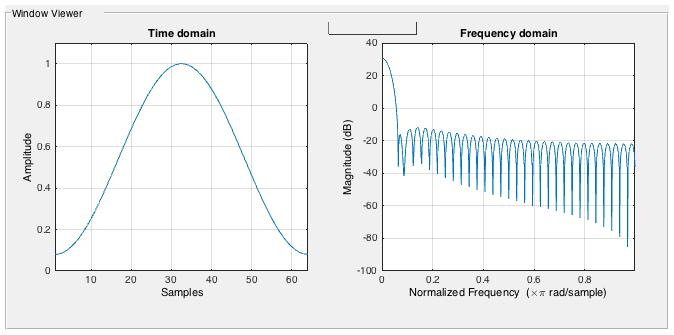
Because of the inherent property of the Hamming window (fixed side lobe), sometimes the signal can get masked.

clear; close all; clc

load winType;

figure;
pwelch(s,[],[],[],Fs);
title('pwelch with default input- f1: 500Hz, f2: 5kHz')
set(gca,'YLim',[-90,0])
set(gca,'XLim',[0,10])
saveas(gcf,'pwelchComplexDefaultPlot.jpg')

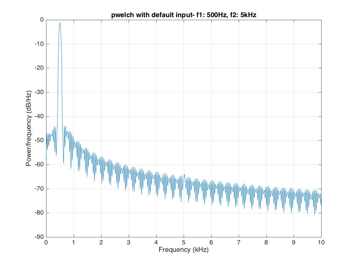
In the above figure, we can see that the signal’s frequency component at 5kHz is barely distinguishable. To resolve this component of frequency, we use the Kaiser window instead of the default Hamming window.

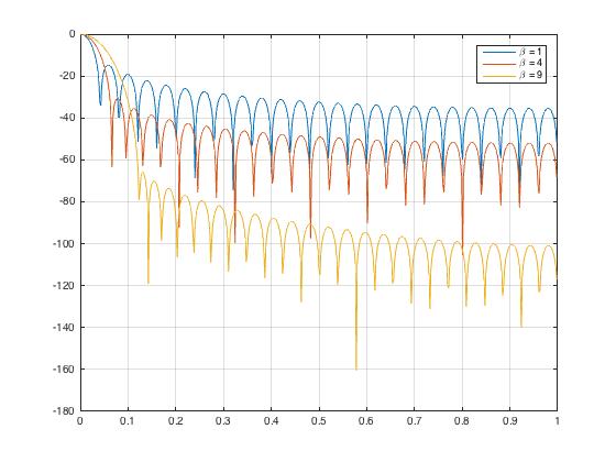
Kaiser Window in Frequency domain

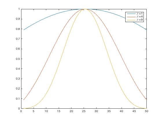
Kaiser Window in time domain

% %% Kaiser window
figure;
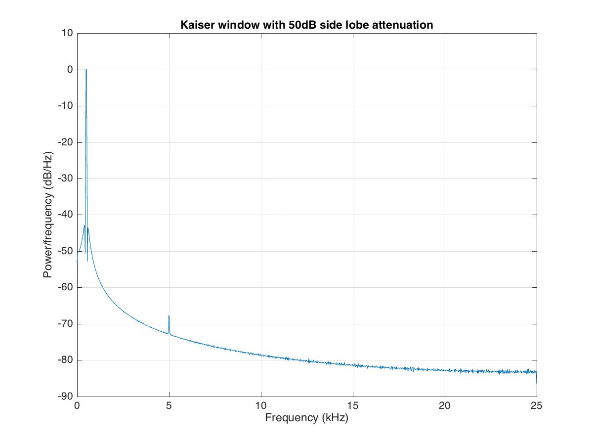
len=2050;
h1=kaiser(len,4.53); %side lobe attenuation of 50dB
pwelch(s,h1,[],len,Fs);
title('Kaiser window with 50dB side lobe attenuation')
saveas(gcf,'pwelchComplexKaise50dBsidelobe.jpg')

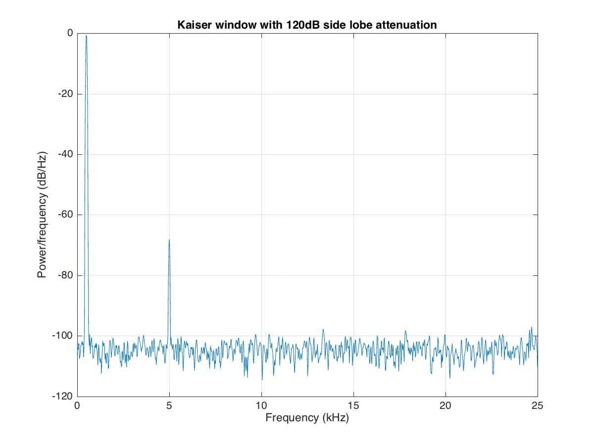
% %% Kaiser window
figure;
len=2050;
h2=kaiser(len,12.26); %side lobe attenuation of 50dB
pwelch(s,h2,[],len,Fs);
title('Kaiser window with 120dB side lobe attenuation')
saveas(gcf,'pwelchComplexKaise120dBsidelobe.jpg')

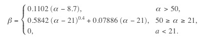
To obtain a Kaiser window that designs an FIR filter with sidelobe attenuation of α dB, we use the following β : kaiser(len,beta)

Amplitude of one frequency component is much lower than the other

We can have some signal where one frequency component’s amplitude is much lower than the others and is inundated in noise. To deal with such signals, we need to get rid of the noise using the window’s averaging.

clear; close all; clc
load winAvg;

% %% Kaiser window
figure;
len=2050;
h1=kaiser(len,4.53); %side lobe attenuation of 50dB
pwelch(s,h1,[],len,Fs);
set(gca,'XLim',[8,18]);
set(gca,'YLim',[-60,-20]);
title('Kaiser window with 50dB side lobe attenuation')
saveas(gcf,'pwelchAvgComplexKaise50dBsidelobe.jpg')

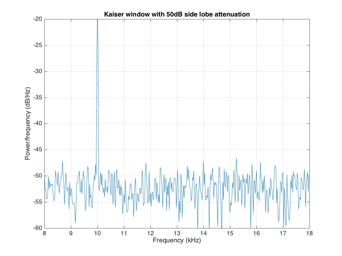
In the above signal plot, the second frequency component at 14kHz is undetectable. We can get rid of the noise using the averaging approach.

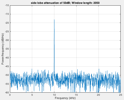
figure;
filename = 'pwelchAveraging.gif';
for len=2050:-100:550
  h2=kaiser(len,4.53); %side lobe attenuation of 50dB
  pwelch(s,h2,[],len,Fs);
  drawnow;
  frame = getframe(1);
   im = frame2im(frame);
   [imind,cm] = rgb2ind(im,256);
   if len == 2050;
     imwrite(imind,cm,filename,'gif', 'Loopcount',inf);
   else
     imwrite(imind,cm,filename,'gif','WriteMode','append');
   end
end

Here, we take the smaller window in steps to show the effect of averaging. A smaller window in the frequency domain is equivalent to the larger window in the time domain.

Dealing with data having missing samples

clear; close all; clc
%%Signals having missing samples
load weightData;
plot(1:length(wgt),wgt,'LineWidth',1.2)
ylabel('Weight in kg'); xlabel('Day of the year')
grid on; axis tight; title('Weight readings of a person')
saveas(gcf,'weightReading.jpg')

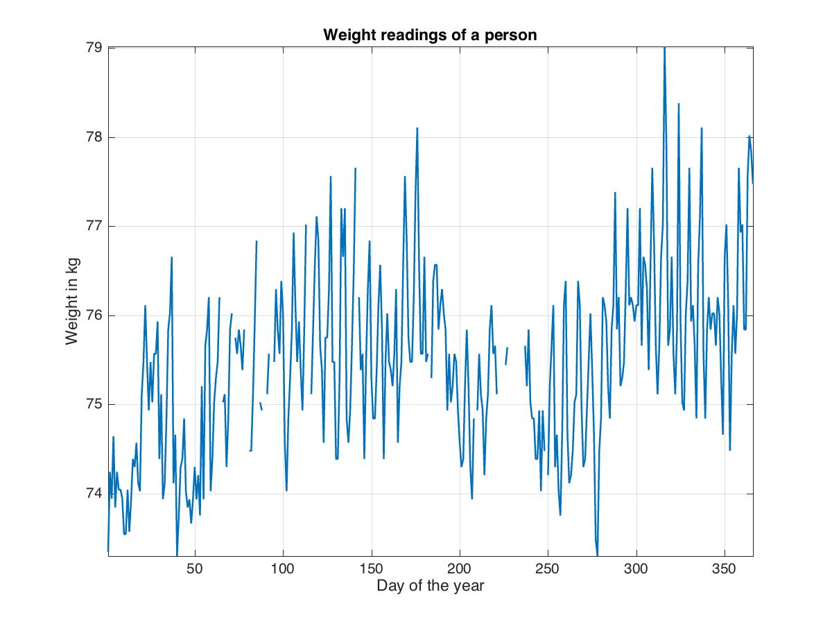
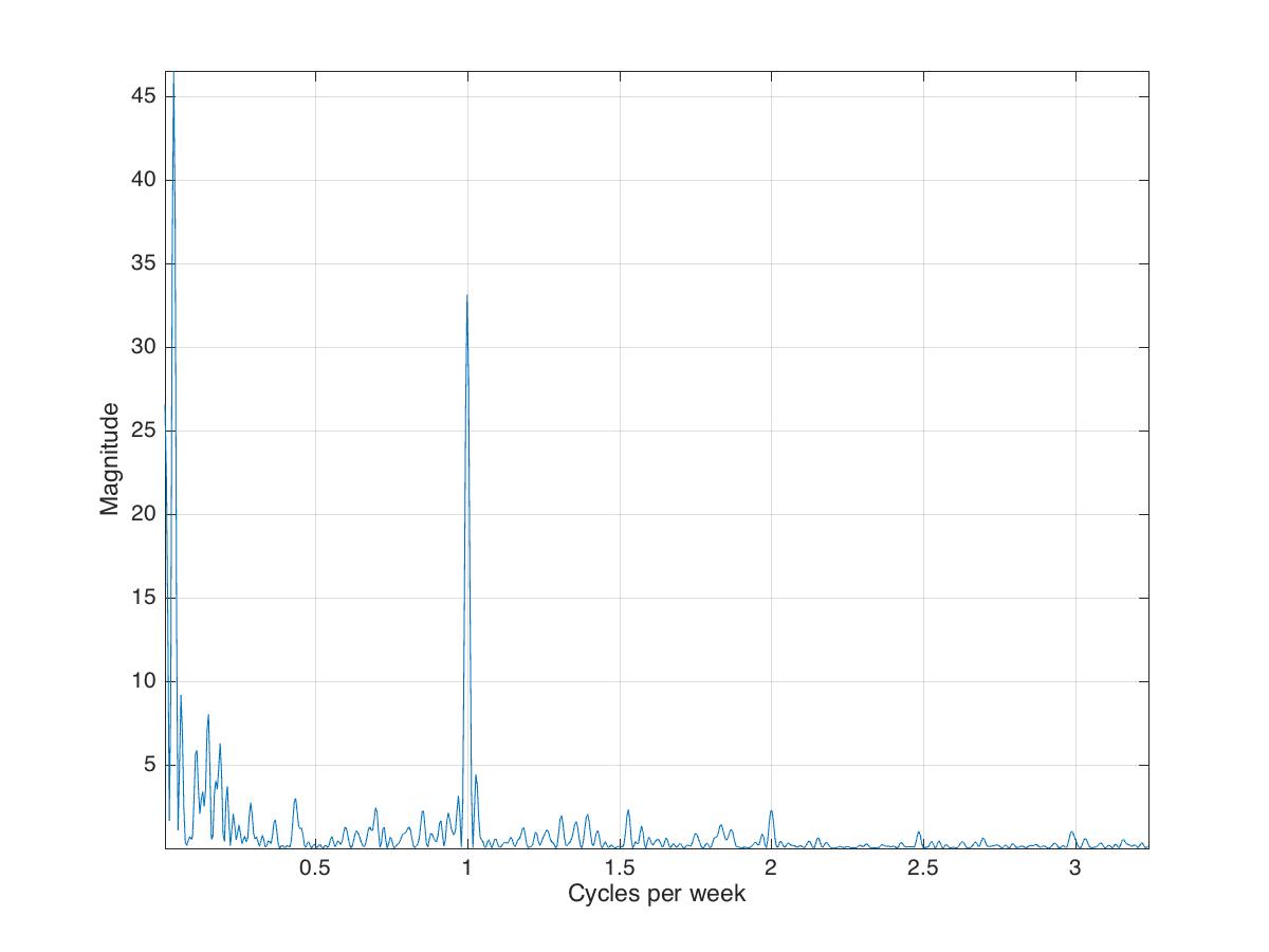
In case we have missing samples in the data, i.e., the data is not regularly recorded, then we cannot apply the “pwelch” function of Matlab to retrieve its frequency components. But thankfully, we have the function “plomb” which can be applied in such cases.

figure;
[p,f]=plomb(wgt,7,'normalized');
plot(f,p)
xlabel('Cycles per week');ylabel('Magnitude')
grid on; axis tight
saveas(gcf,'plombspectrum.jpg')

Analyzing time and frequency domain simultaneously

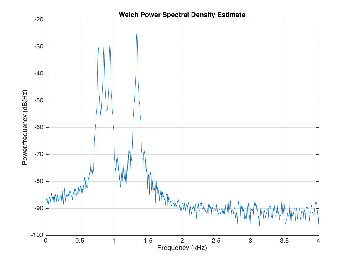
Sometimes, we need time and frequency information simultaneously. For a long series of data, we need to know which frequency component is recorded first and at what time. This can be done by making the spectrogram.

clear; close all; clc
load dtmf;

%%
figure;
pwelch(x,[],[],[],Fs)
saveas(gcf,'powerspectrum_dtmf.jpg')

% %%
figure;
spectrogram(x,[],[],[],Fs,'yaxis'); colorbar; %default window is hamming window
saveas(gcf,'spectrogramDefault_dtmf.jpg')

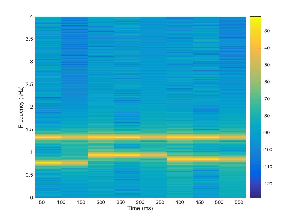
Since the time resolution is higher for smaller windows and frequency resolution is lower at small window length. So there is a trade-off between the time and frequency domain window length. We need to figure out the optimal point for better resolution in both the time and frequency domain.

segLen = [120, 240,480,600,800,1000,1200,1600];

figure;
filename='spectrogramAnalysis.gif';
for itr = 1:numel(segLen)
 spectrogram(x,segLen(itr),[],segLen(itr),Fs,'yaxis');
 set(gca,'YLim',[0,1.7]);
 title(sprintf('window length: %d',segLen(itr)))
 colorbar;
 drawnow;
 frame = getframe(1);
 im = frame2im(frame);
 [imind,cm] = rgb2ind(im,256);
 if itr == 1;
 imwrite(imind,cm,filename,'gif', 'Loopcount',inf);
 else
 imwrite(imind,cm,filename,'gif','WriteMode','append');
 end
end

Recap

• fft gives the overall magnitude and phase spectrum — which frequencies, not when.
• pwelch (Welch’s method) estimates the power spectral density by averaging windowed FFTs of overlapping segments, trading a little resolution for a much smoother, lower-variance estimate.
• Window length is the key knob: a long window resolves close frequencies (fine frequency resolution) but blurs timing; a short window does the reverse. You can’t sharpen both — the uncertainty principle.
• The window shape matters too: a Kaiser window (with an adjustable beta) lets you trade main-lobe width against sidelobe attenuation to uncover a weak component next to a strong one.
• For irregularly sampled data, pwelch won’t work — use plomb (Lomb–Scargle). For a joint time × frequency view, use spectrogram, and animate over window lengths to find the sweet spot.

Where to go next

• Signal denoising using the Fast Fourier Transform — put the spectrum to work removing noise.
• Towards multi-resolution analysis with the wavelet transform — wavelets adapt the window automatically, sidestepping the fixed-window trade-off.
• Concatenating daily seismic traces and plotting a spectrogram — the same spectrogram idea applied to real seismic data in Python.