Getting started with Obspy: Downloading waveform data (codes included)
Obspy is getting popular everyday among seismologists for data analysis and for quick visualization in some cases. But I found that it is still difficult for some researchers to transition from traditional tools like SAC, SEISAN, etc to modern and flexible Obspy. The main reason is not the complexity of Obspy but their unfamiliarity to Python. Python adds immense dynamics and flexibility to Obspy. In my opinion, the greatest feature of Python is to act as a wrapper for all major programming languages and also provide the native capability to perform all sorts of mathematical and graphical operations. Obspy plays on the strength of Python. In this post, I will introduce how to use Obspy along with some details of the required Python steps.
Introduction
Obspy is an open-source Python framework developed for the processing of seismological data. The strength of Obspy is that it works with several file formats, contains modules for accessing data from several open-access data centers and has modules for routine seismological processing.
Key idea — a SEED id plus a time window fetches a seismogram. To download data you tell an FDSN client four codes — network, station, location, channel (the SEED identifier) — and a start/end time (via UTCDateTime). client.get_waveforms(...) returns a Stream: a list-like container of Trace objects, each a numpy data array plus a Stats header (station, channel, sampling rate, start time). From there you plot() it, remove_response() to get real ground motion, filter(), and write() it to disk. The metadata carried in every Trace is what makes it seismology, not just numbers.
Installation
If you do not have Obspy installed in your computer then you can install following these steps. I recommend installation via Anaconda.
For this tutorial, you can install all the necessary libraries using the environment file:
![]()
For installing the environment with all the libraries:
conda env create -f earthinversion_env.yml
Then you can activate the environment:
conda activate earthinversion
Example 1: Downloading waveform data for a particular station
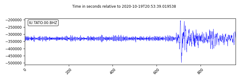
Obspy can download waveform data from open-access data centers using the specified details. For this example, we arbitrarily select the recent major earthquake “2020-10-19 Mww7.6 South Of Alaska”. We select the station: IU.TATO (Taipei, Taiwan).
First we import all the necessary modules:
from obspy import read
from obspy.clients.fdsn import Client
from obspy import UTCDateTime
import matplotlib.pyplot as plt
Then we set IRIS as our client for downloading data. There are several other data clients available. For more visit this page.
client = Client(
   "IRIS"
)
“IRIS” is now EarthScope — but the code still works. In 2023 the IRIS Data Management Center merged into the EarthScope Consortium. The Client("IRIS") shortcut still resolves (ObsPy keeps it as an alias to the same FDSN web service), so nothing here breaks. You may also see Client("EARTHSCOPE") and the newer service.iris.edu / EarthScope endpoints in current docs — they point at the same archive.
Now, let us select a station for downloading the data. In practice you may wanna select the event first and then search for all the available stations for that event. We will look into that case later.
net = "IU"  # network of the station
sta = "TATO"  # station code
loc = "00"  # to specify the instrument at the station
chan = "BHZ"
Let us download the data for 2020-10-19 Mww7.6 South Of Alaska earthquake. We can specify the event using the time range within which the event falls. Obspy uses UTCDateTime module for that (not to be confused with the datetime. module, which has similar functions.
We first define the event time and then define the start and end time of the waveforms to request. Here, we will request waveforms one minute before the origin time and 15 minutes after the origin time.
eventTime = UTCDateTime("2020-10-19T20:54:39")
starttime = eventTime - 60  # 1 minute before the event
endtime = eventTime + 15 * 60  # 15 minutes after the event
Now, we download the waveforms and store it into a Stream object. Streams are list-like objects which contain multiple Trace objects, i.e. gap-less continuous time series and related header/meta information.
myStream = client.get_waveforms(net, sta, loc, chan, starttime, endtime)
print(myStream)
1 Trace(s) in Stream:
IU.TATO.00.BHZ | 2020-10-19T20:53:39.019538Z - 2020-10-19T21:09:38.969538Z | 20.0 Hz, 19200 samples
We can see that the stream contains one trace because we requested only one waveforms corresponding to one channel. Next, we would like to inspect the contents of this stream. We can have quick interactive plot of the stream using the plot method.
myStream.plot()
If you want to save the plot, you can redirect the plot to file using the outfile argument. We can also select the starttime and endtime of the plot to hide other parts in the original waveform. Besides, we can perform several other modifications using the arguments in the plot method.
myStream.plot(
    outfile="myStream.png",
    starttime=None,
    endtime=None,
    size=(800, 250),
    dpi=100,
    color="blue",
    bgcolor="white",
    face_color="white",
    transparent=False,
    number_of_ticks=6,
    tick_rotation=45,
    type="relative",
    linewidth=0.5,
    linestyle="-",
)
Obspy can output into formats such as png, pdf, ps, eps and svg. The type argument specifies the type of plot. There are several type of the plot in Obspy but in general there are two: normal or relative. The different is in the x-axis display of time.
Next step is to write the downloaded data into a file for later use. We can do this using the write method of stream object.
myStream.write("myStream.mseed", format="MSEED")
Obspy supports several other file formats.
Complete script for downloading data and plotting
Complete script for downloading all broadband components
Example 2: Download vertical component waveforms, remove instrument response and plot
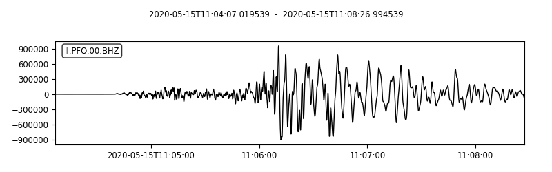
I will download the seismic time series recording a major earthquake. I will use the Obspy module to download the data from IRIS. I will download the waveforms for the arbitrarily selected event “2020-05-15 Mww 6.5 Nevada” located at (38.1689°N, 117.8497° W).
from obspy import read
from obspy.clients.fdsn import Client
from obspy import UTCDateTime
import matplotlib.pyplot as plt

client = Client("IRIS")

origin_time = UTCDateTime("2020-05-15T11:03:27Z")
net = "II"
stn = "PFO"
channel = "BHZ"
st = client.get_waveforms(net, stn, "00", channel,
                          origin_time+40, origin_time+300, attach_response=True)
st_copy = st.copy()
st_copy.remove_response(output="VEL")

# Filtering with a lowpass on a copy of the original Trace
st_copy[0].filter('highpass', freq=5.0, corners=2, zerophase=True)

st.plot(
    outfile="myStream.png",
)

print(st_copy)
st.write(f'{net}-{stn}-{channel}.mseed', format="MSEED")
1 Trace(s) in Stream:
II.PFO.00.BHZ | 2020-05-15T11:04:07.019539Z - 2020-05-15T11:08:26.994539Z | 40.0 Hz, 10400 samples
This saves the mseed data into the script directory as well the plot of the “stream”. I also highpass filtered the signal to obtain the high-frequency part of the time series.
See my other posts for denoising the seismic waveforms using Fourier Transform (low-pass filter), or using wavelet-based advanced techniques.
Quick check: What does client.get_waveforms("IU", "TATO", "00", "BHZ", starttime, endtime) return?
- A single numpy array of samples with no metadata
- A
Streamobject containing one or moreTraces, each with a data array and aStatsheader - A PNG image of the waveform
- The raw bytes of a miniSEED file
Recap
- ObsPy downloads seismic data through an FDSN client: pick a data center (
Client("IRIS")), give it a SEED id (network, station, location, channel) and a time window (UTCDateTime), and callget_waveforms(...). - The result is a
StreamofTraces — each a numpy data array plus aStatsheader. Inspect it by printing (print(myStream)) or plotting (myStream.plot(...)). remove_response(output="VEL")converts raw counts to true ground motion (needs the response, e.g.attach_response=True);filter(...)applies band-pass/high-pass filtering.write("...mseed", format="MSEED")saves the data — swap the format string for SAC and others.- “IRIS” is now EarthScope (2023 merger); the
Client("IRIS")alias still works.
Where to go next
- Plotting a record section with ObsPy — visualize many stations at once.
- Automatically enquire seismic data availability with ObsPy — find which stations recorded an event before downloading.
- Signal denoising using the Fast Fourier Transform — clean up the waveforms you fetched.
Disclaimer of liability
The information provided by the Earth Inversion is made available for educational purposes only.
Whilst we endeavor to keep the information up-to-date and correct. Earth Inversion makes no representations or warranties of any kind, express or implied about the completeness, accuracy, reliability, suitability or availability with respect to the website or the information, products, services or related graphics content on the website for any purpose.
UNDER NO CIRCUMSTANCE SHALL WE HAVE ANY LIABILITY TO YOU FOR ANY LOSS OR DAMAGE OF ANY KIND INCURRED AS A RESULT OF THE USE OF THE SITE OR RELIANCE ON ANY INFORMATION PROVIDED ON THE SITE. ANY RELIANCE YOU PLACED ON SUCH MATERIAL IS THEREFORE STRICTLY AT YOUR OWN RISK.
Leave a comment