The easy way to compute and visualize the time & frequency domain correlation (codes included)
Introduction
Cross-correlation is an established and reliable tool to compute the degree to which the two seismic time-series are dependent on each other. Several studies have relied on the cross-correlation method to obtain the inference on the seismic data. For details on cross-correlation methods, we refer the reader to previous works [see references].
It is essential to understand and identify the complex and unknown relationships between two time-series for obtaining meaningful inference from our data. In this post, we will take the geophysical data for understanding purposes. For general readers, I recommend to ignore the field specific examples and stay along, as the concept of correlation is mathematical and can be applied on data related to any field.
In seismology, several applications are based on finding the time shift of one time-series relative to other such as ambient noise cross-correlation (to find the empirical Green’s functions between two recording stations), inversion for the source (e.g., gCAP) and structure studies (e.g., full-waveform inversion), template matching etc.
In this post, we will see how we can compute cross-correlation between seismic time-series and extract the time-shift information of the relation between the two seismic signals in the time and frequency domain.
Time domain cross-correlation function
The correlation between two-stochastic processes A and B (expressed in terms of time-series as \(A(t)\) and \(B(t)\)) can be expresses as (see ref. 1):
\begin{equation} \label{eq:square} \begin{split} \rho (\tau) = \frac{\sum_i A(t_i-\tau) B(t_i)}{[\sum_i A(t_i)^2\sum_iB(t_i)^2]^{1/2}} \end{split} \end{equation}
The above equation is the sample cross-correlation function between two time-series with a finite time shift \(\tau\). It is important to note that the correlation \(\rho\) by its face value alone does not dictate whether or not the correlation in question is significant, unless the degrees of freedom (DOF) of the processes, which signifies the information content (or entropy), is also specified (see Chao and Chung, 2019 for details).
Compute Cross-correlation
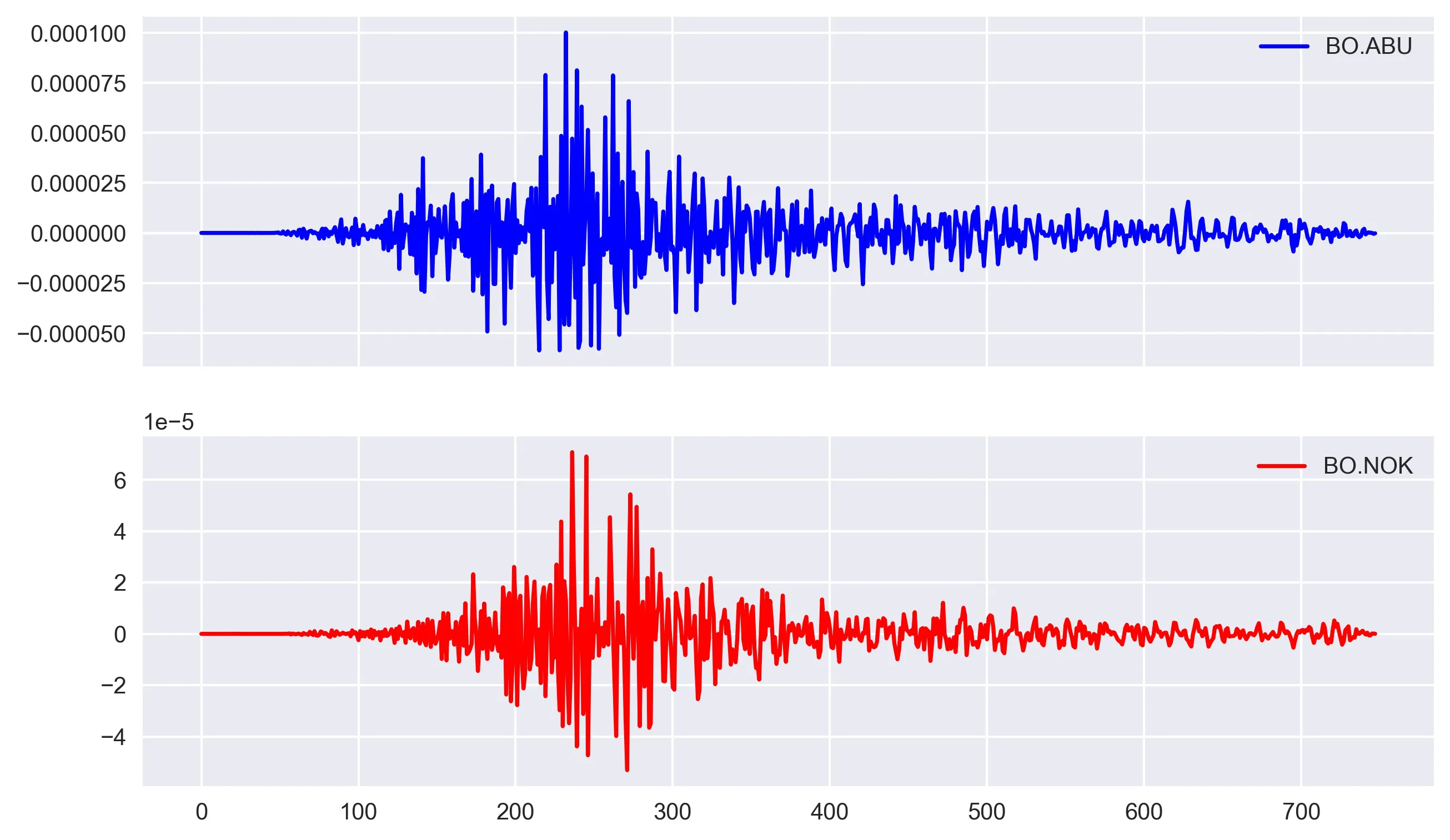
Let us now look into how we can compute the time domain cross correlation between two time series. For this task, I arbitrarily took two seismic velocity time-series:
Arbitrarily selected data
import numpy as np
import matplotlib.pyplot as plt
import pandas as pd
from synthetic_tests_lib import crosscorr


time_series = ['BO.ABU', 'BO.NOK']
dirName = "data/"
fs = 748  # take 748 samples only
MR = len(time_series)
Y = np.zeros((MR, fs))
dictVals = {}
for ind, series in enumerate(time_series):
    filename = dirName + series + ".txt"
    df = pd.read_csv(filename, names=[
                     'time', 'U'], skiprows=1, delimiter='\s+')  # reading file as pandas dataframe to work easily

    # this code block is required as the different time series has not even sampling, so dealing with each data point separately comes handy
    # can be replaced by simply `yvalues = df['U]`
    yvalues = []
    for i in range(1, fs+1):
        val = df.loc[df['time'] == i]['U'].values[0]
        yvalues.append(val)

    dictVals[time_series[ind]] = yvalues


timeSeriesDf = pd.DataFrame(dictVals)
The above code reads the txt file containing the vertical component located in the directory (dirName) and trim the data for arbitraily taken fs samples. We can read each txt file interatively and save the data column into a dictionary. This dictionary is next converted into pandas dataframe to avail all the tools in pandas library.
The above code reads the txt file containing the vertical component located in the directory (dirName) and trim the data for arbitraily taken fs samples. We can read each txt file interatively and save the data column into a dictionary. This dictionary is next converted into pandas dataframe to avail all the tools in pandas library.
Please note that there are several different ways to read the data and preference of that way depends on the user and the data format.
To plot the time-series, I used matplotlib.
# plot time series
# simple `timeSeriesDf.plot()` is a quick way to plot
fig, ax = plt.subplots(2, 1, figsize=(10, 6), sharex=True)
ax[0].plot(timeSeriesDf[time_series[0]], color='b', label=time_series[0])
ax[0].legend()
ax[1].plot(timeSeriesDf[time_series[1]], color='r', label=time_series[1])
ax[1].legend()
plt.savefig('data_viz.jpg', dpi=300, bbox_inches='tight')
plt.close('all')
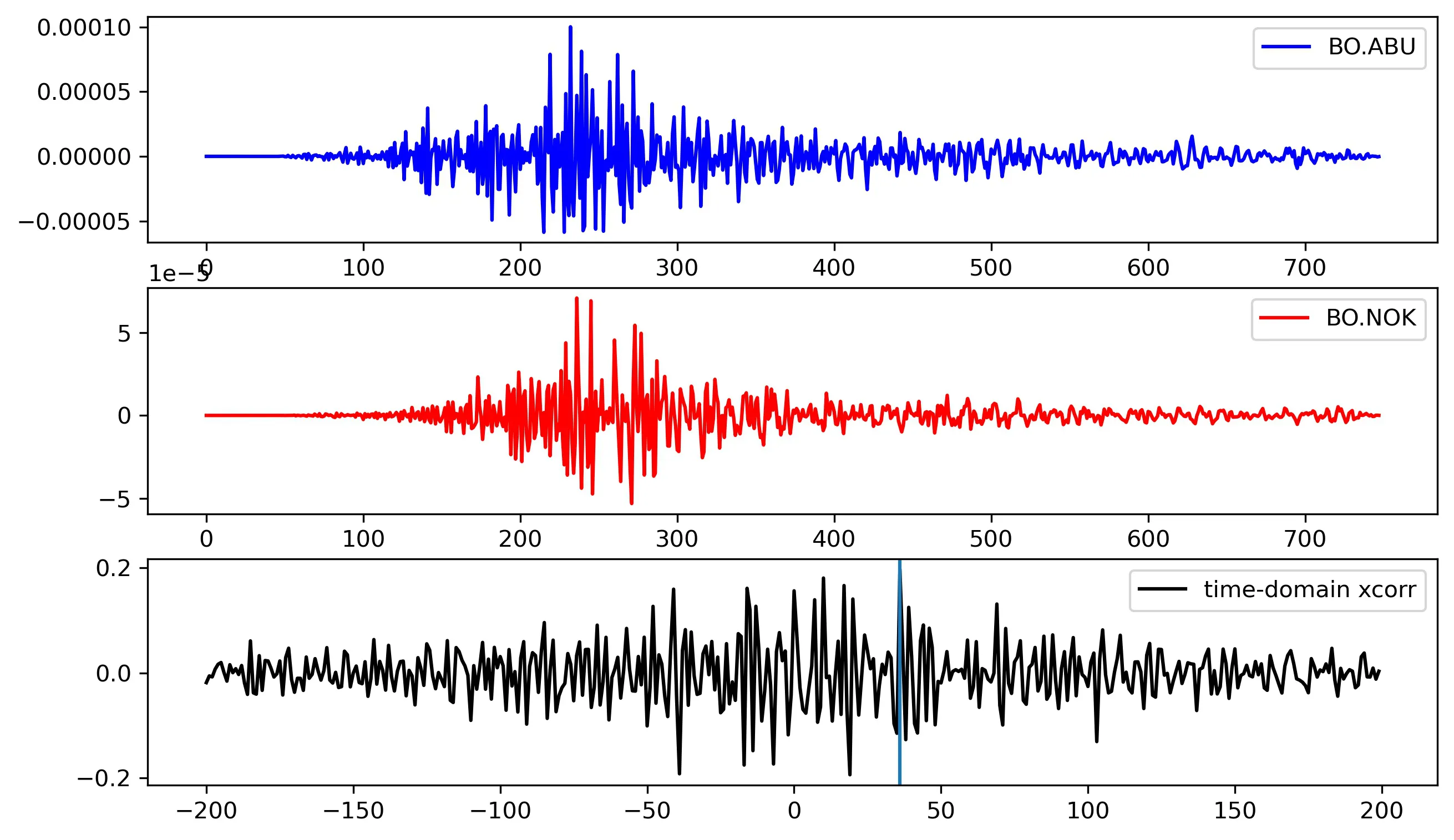
Compute the cross-correlation in time-domain
d1, d2 = timeSeriesDf[time_series[0]], timeSeriesDf[time_series[1]]
window = 10
# lags = np.arange(-(fs), (fs), 1)  # uncontrained
lags = np.arange(-(200), (200), 1)  # contrained
rs = np.nan_to_num([crosscorr(d1, d2, lag) for lag in lags])

print(
    "xcorr {}-{}".format(time_series[0], time_series[1]), lags[np.argmax(rs)], np.max(rs))
In this example, timeSeriesDf[time_series[0]], and timeSeriesDf[time_series[1]] are the two pandas Series object as required by the crosscorr function. I read the time series from the Pandas DataFrame timeSeriesDf, for the specified columns time_series[ind1] and time_series[ind2], where time_series is a list with two elements.
Alternatively, one can directly create Pandas Series object by using pd.Series().
I have used the crosscorr function to compute the correlation between the pair of time-series for a series of lag values. The lag values has been contrained between -200 to 200 to avoid artifacts.
# Time lagged cross correlation
def crosscorr(datax, datay, lag=0):
    """ Lag-N cross correlation.
    Shifted data filled with NaNs

    Parameters
    ----------
    lag : int, default 0
    datax, datay : pandas.Series objects of equal length
    Returns
    ----------
    crosscorr : float
    """
    return datax.corr(datay.shift(lag))
Here, as you can notice that the crosscorr makes use of the pandas corr method and hence, the d1 and d2 is required to be pandas Series object.
I obtained the correlation between the above pair of time-series to be 0.19with a lag of 36.
xcorr BO.ABU-BO.NOK 36 0.19727959397327688
Frequency-domain approach of cross-correlation for obtaining time shifts
shift = compute_shift(
    timeSeriesDf[time_series[0]], timeSeriesDf[time_series[1]])

print(shift)
This gives:
-36
Where, the function compute_shift is simply:
def cross_correlation_using_fft(x, y):
    f1 = fft(x)
    f2 = fft(np.flipud(y))
    cc = np.real(ifft(f1 * f2))
    return fftshift(cc)

def compute_shift(x, y):
    assert len(x) == len(y)
    c = cross_correlation_using_fft(x, y)
    assert len(c) == len(x)
    zero_index = int(len(x) / 2) - 1
    shift = zero_index - np.argmax(c)
    return shift
Here, the shift of shift means that y starts shift time steps before x.
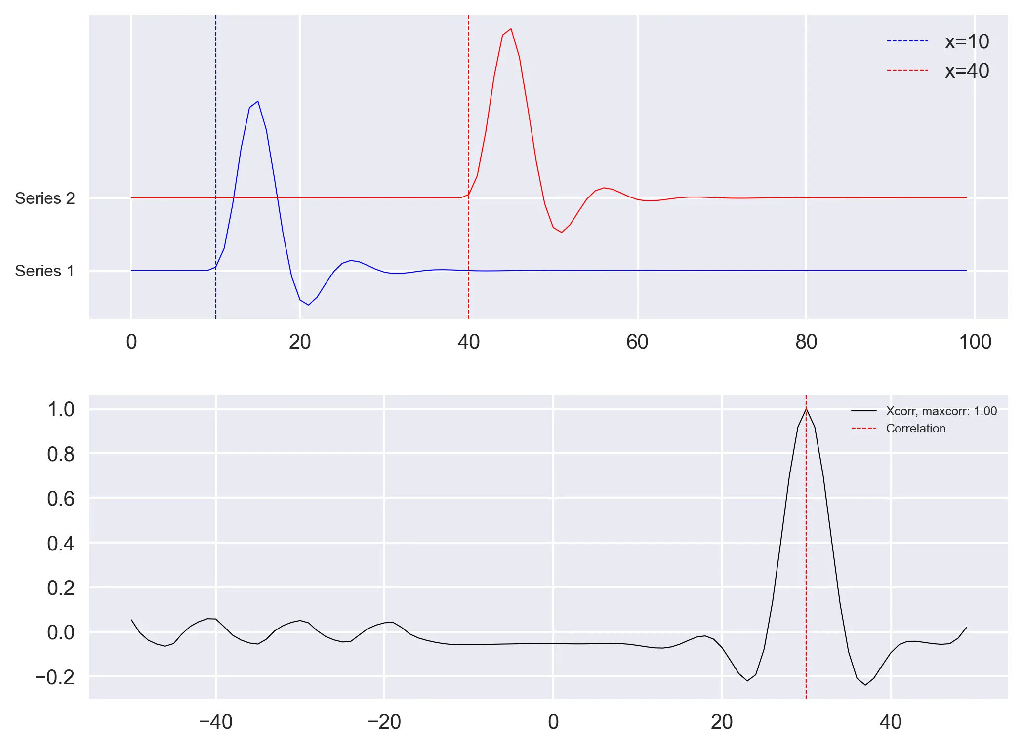
Generate synthetic pair of time series
Although the results obtained seems plausible, as we used the arbitrary pair of real time series, we do not know if we have obtained the correct results. So, we apply the above methods on synthetic pair of time-series with known time-shifts.
Let us use the scipy.signal fucntion to generate two unit impulse function. We then apply low pass filter of order 4 and with center frequency of 0.2 to smoothen the edges (Note that the results will be same even without the filter).
# Delta Function
length = 100
amp1, amp2 = 1, 1
x = np.arange(0, length)
to = 10
timeshift = 30
t1 = to+timeshift
series1 = signal.unit_impulse(length, idx=to)
series2 = signal.unit_impulse(length, idx=t1)

# low pass filter to smoothen the edges (just to make the signal look pretty)
b, a = signal.butter(4, 0.2)
series1 = signal.lfilter(b, a, series1)
series2 = signal.lfilter(b, a, series2)

fig, ax = plt.subplots(2, 1, figsize=(8, 6), sharex=False)

ax[0].plot(x, series1, c='b', lw=0.5)
ax[0].axvline(x=to, c='b', lw=0.5,
              ls='--', label=f'x={to}')
ax[0].plot(x, series2+0.1, c='r', lw=0.5)
ax[0].axvline(x=to+timeshift, c='r', lw=0.5,
              ls='--', label=f'x={to+timeshift}')
ax[0].set_yticks([0, 0.1])
ax[0].legend()
ax[0].set_yticklabels(['Series 1', 'Series 2'], fontsize=8)

d1, d2 = pd.Series(series2), pd.Series(series1)
lags = np.arange(-(50), (50), 1)

rs = np.nan_to_num([crosscorr(d1, d2, lag) for lag in lags])
maxrs, minrs = np.max(rs), np.min(rs)
if np.abs(maxrs) >= np.abs(minrs):
    corrval = maxrs
else:
    corrval = minrs

ax[1].plot(lags, rs, 'k', label='Xcorr (s1 vs s2), maxcorr: {:.2f}'.format(
    corrval), lw=0.5)
# ax[1].axvline(x=timeshift, c='r', lw=0.5, ls='--')
ax[1].axvline(x=lags[np.argmax(rs)], c='r', lw=0.5,
              ls='--', label='max time correlation')
ax[1].legend(fontsize=6)
plt.subplots_adjust(hspace=0.25, wspace=0.1)
plt.savefig('xcorr_fn_delta.png', bbox_inches='tight', dpi=300)
plt.close('all')
References
- Chao, B.F., Chung, C.H., 2019. On Estimating the Cross Correlation and Least Squares Fit of One Data Set to Another With Time Shift. Earth Sp. Sci. 6, 1409–1415. https://doi.org/10.1029/2018EA000548
- Robinson, E., & Treitel, S. (1980). Geophysical signal analysis. Englewood Cliffs, NJ: Prentice‐Hall.
- Template matching using fast normalized cross correlation
- Qingkai’s Blog: “Signal Processing: Cross-correlation in the frequency domain”
- How to Calculate Correlation Between Variables in Python
Download Codes
All the above codes can be downloaded from my Github repo.
Disclaimer of liability
The information provided by the Earth Inversion is made available for educational purposes only.
Whilst we endeavor to keep the information up-to-date and correct. Earth Inversion makes no representations or warranties of any kind, express or implied about the completeness, accuracy, reliability, suitability or availability with respect to the website or the information, products, services or related graphics content on the website for any purpose.
UNDER NO CIRCUMSTANCE SHALL WE HAVE ANY LIABILITY TO YOU FOR ANY LOSS OR DAMAGE OF ANY KIND INCURRED AS A RESULT OF THE USE OF THE SITE OR RELIANCE ON ANY INFORMATION PROVIDED ON THE SITE. ANY RELIANCE YOU PLACED ON SUCH MATERIAL IS THEREFORE STRICTLY AT YOUR OWN RISK.
Leave a comment