Numerical Tests on Travel Time Tomography [MATLAB]
Introduction
Tomography, which is derived from the Greek word “tomos” that is “slice”, denotes forming an image of an object from measurements made from slices or rays through it. In other words, forming the structure of an object based on a collection of slices through it.
In principle, it is usually an inverse problem where we have the data, we formulate the geometry of the ray paths and invert for the model parameters that defines the structure.
\[\begin{aligned} d &= Gm \end{aligned}\]where, \( d \) is the vector containing the data, \( m \) is the vector containing the model parameters and \( G \) is the kernel which maps the data into the model and vice-versa. If there are \( N \) number of data and \( M \) number of model parameters then the size of the matrix \( G \) is \( N \times M \).
The first step of this problem is to formulate a theoretical relationship between the data and model spaces and the underlying physics. Once, this theoretical relationship is established or the matrix \( G \) is formulated, we can address the above problem in two ways – a forward problem or an inverse problem.
The forward problem can be taken as a trial and error process or as an exhaustive search through the model space for the best set of model parameters which can reduce the misfit between the observed and the predicted data. For this case, we guess the model based on the simple real world geology and then determine the data based on the theoretical relationship between data and models. In contrast, in the inverse problem we invert for the model parameters using the data and considering the theoretical relationship between the data and model parameters. Then we interpret for the real world geology.
The solution of the linear tomographic inverse problem depends on the relationship between \( N \) and \( M \). If \( N \) < \( M \), then we have more number of model parameters or variables to obtained and lesser number of data or equations to solve. In this case, the equation \( d = Gm \) does not provide enough information to determine uniquely all the model parameters and thus the problem is called underdetermined. We usually need extra constraints to solve this kind of problem, for example we take the a priori constraint that the solution to this problem is simple. If \( N = M \), then there is ideally enough information to determine the model parameters. But in real world, data is usually inaccurate and inconsistent to invert for the best model parameters in this case. If \( N > M \), there is too much information contained in the equation \( d = Gm \) for it to possess an exact solution. This case is called the overdetermined.
Solution of the underdetermined linear inverse problem:
We take the a priori constraint that the solution is simple. The notion of simplicity is quantified by some measure of the length of the solution. One such measure is the Euclidean length of the solution, \( L = m^{T}m \).
\[\begin{aligned} d &= Gm \\ 𝑚^{est} &= 𝐺^T(𝐺𝐺^T)^{-1}𝑑 \end{aligned}\]Solution of the overdetermined linear inverse problem:
\[\begin{aligned} d &= Gm \\ 𝑚^{est} &= (𝐺^T𝐺)^{-1}𝐺^T𝑑 \end{aligned}\]This solution can simply be obtained simply by minimizing the least square error with respect to the model parameters. (Menke 1989)
Solution of the Mixed-Determined linear inverse problem:
Most inverse problems that arise in practice are neither completely overdetermined nor completely underdetermined. So, for solving these kinds of problems, ideally we would like to sort the unknown model parameters into two groups- overdetermined and underdetermined. For doing so, we form a set of new model parameters that are linear combinations of the old. Then we can partition from an arbitrary \( d = Gm \) to \( d’ = G’m’ \), where \( m’ \) is partitioned into an upper part that is overdetermined and a lower part that is underdetermined.
\[\begin{bmatrix} G^{'o} & 0 \\ 0 & G^{'o} \end{bmatrix} \begin{bmatrix} m^{'o} \\ m^{'u} \end{bmatrix} = \begin{bmatrix} d^{'o} \\ d^{'u} \end{bmatrix}\]This partitioning process can be accomplished through singular value decomposition of the data kernel. If this can be achieved then we can determine the overdetermined model parameters by solving the upper equations in the least square sense and determine the underdetermined model parameters by finding those that have minimum least square solution length.
Instead of partitioning \( m \), we can determine the solution that minimizes some combination \( \phi \) of the prediction error and the solution length for the model parameters.
\[\phi (m) = (𝑑−𝐺𝑚)^{T} (𝑑−𝐺𝑚) +\epsilon^2 𝑚^T𝑚\]The weighting parameter \( \epsilon^2 \) determines the relative importance given to the prediction error and solution length. There is no simple method of determining the value of \( \epsilon \) and it should be determined using the hit-and-trial method. By minimizing the \( \phi (m) \) , we obtain
\[m^{est} = (G^TG+\epsilon^2I)^{-1}G^Td\]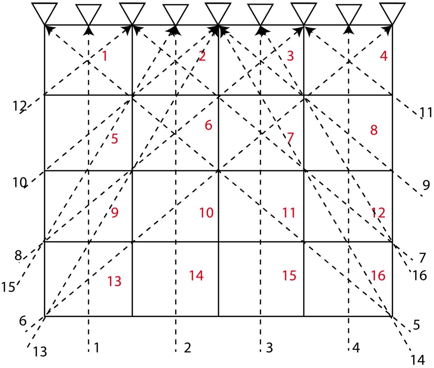
A Simple Tomography Model
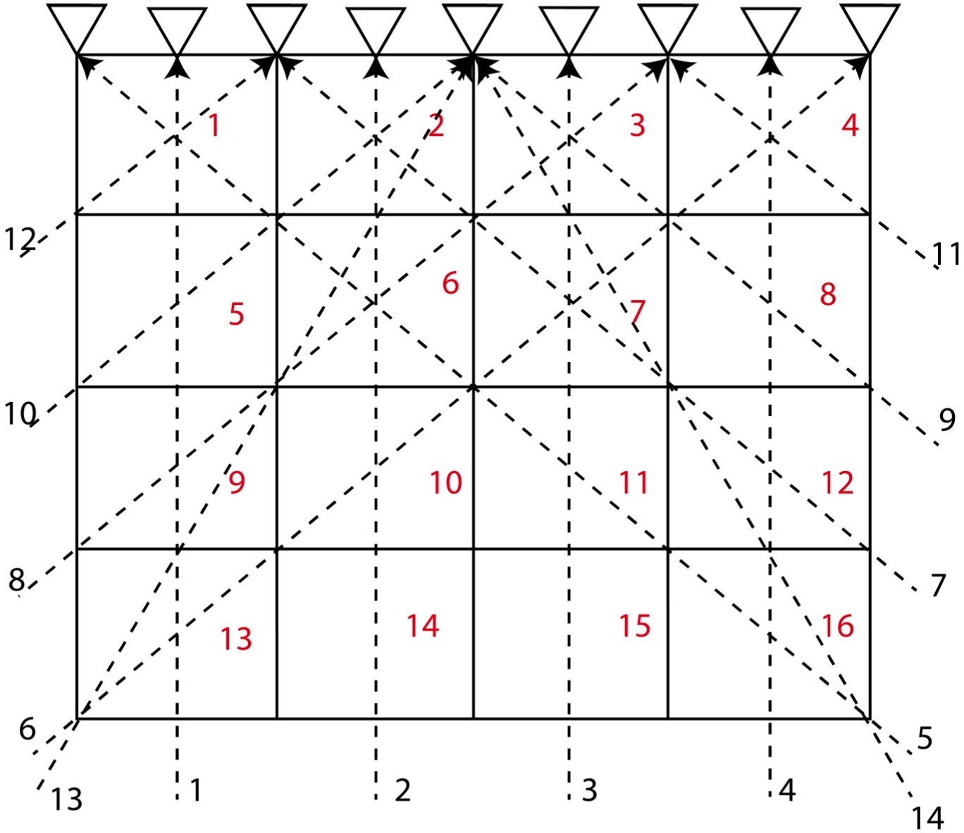
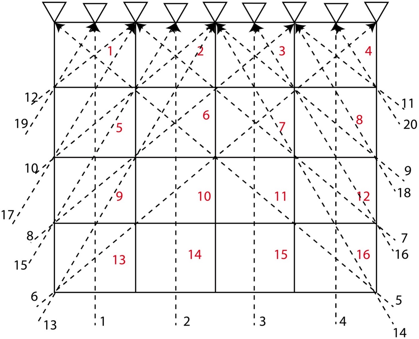
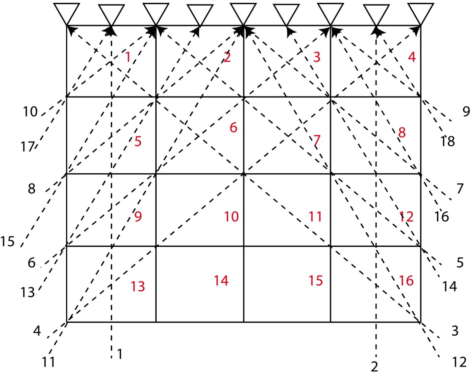
Let us consider a 2D structure for which we want to determine the model parameters. To invert for the model parameters, we divide the whole 2D region into 4 cells (2*2). We consider that the velocity of different cells differ, so we might attempt to distinguish the velocity or model parameter for each cell by measuring the travel time of the rays across the various rows and columns of the cells.
In this problem, we consider 4 cells and 6 travel time data (or rays) and hence \( M = 4 \) and \( N = 6 \). Here, we assume that the velocity for each cell is uniform and that the travel time of the ray across each cell is proportional to the width and height of the cell. Instead of considering the velocity as our model parameters, we consider slowness \( \frac{1}{velocity} \) as our model parameters. This is because it will reduce the complexity in our equations to solve for the model parameters.
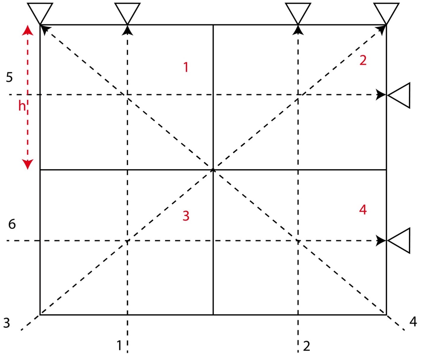
The equations for the different ray paths will be
Ray path 1:
\[𝑔_{11} 𝑚_1 + 𝑔_{12} 𝑚_2 + 𝑔_{13} 𝑚_3 + 𝑔_{14} 𝑚_4 = 𝑑_1\]Ray path 2:
\[𝑔_{21} 𝑚_1 + 𝑔_{22} 𝑚_2 + 𝑔_{23} 𝑚_3 + 𝑔_{24} 𝑚_4 = 𝑑_2\]Ray path 3:
\[𝑔_{31} 𝑚_1 + 𝑔_{32} 𝑚_2 + 𝑔_{33} 𝑚_3 + 𝑔_{34} 𝑚_4 = 𝑑_3\]Ray path 4:
\[𝑔_{41} 𝑚_1 + 𝑔_{42} 𝑚_2 + 𝑔_{43} 𝑚_3 + 𝑔_{44} 𝑚_4 = 𝑑_4\]Ray path 5:
\[𝑔_{51} 𝑚_1 + 𝑔_{52} 𝑚_2 + 𝑔_{53} 𝑚_3 + 𝑔_{54} 𝑚_4 = 𝑑_5\]Ray path 6:
\[𝑔_{61} 𝑚_1 + 𝑔_{62} 𝑚_2 + 𝑔_{63} 𝑚_3 + 𝑔_{64} 𝑚_4 = 𝑑_6\]\
The above 6 equations can be written in the form of
Here, the vector \(d\) contains the travel time data along each ray path. The matrix \(G\) contains the information about the geometry of the ray-path. Here, \(G\) consists of the length of each ray-path in different cells. The vector \(m\) consists of the slowness parameters for each cell.\
Since, this is an over-determined case, we invert for the model parameters using the least square scenario:
\[m^{est} = [G^T G]^{-1} G^T d\]MATLAB CODES for inversion and plotting
clear; close all; clc
N=6; %no. of ray paths
M=4; %no. of model parameters
G=zeros(N,M); %initializing the kernel
h=15; %length of the grid
hh=h*sqrt(2); %length of the diagonal of grid

G=[h 0 h 0; 0 h 0 h; 0 hh hh 0;hh 0 0 hh; h h 0 0; 0 0 h h]; %kernel matrix

mm=[4 7 12 18]'; %actual model parameter - velocity (arbitrarily taken)
m=1./mm; %actual model parameter - slowness

tt=G*m; %actual travel time at the stations
[nt,mt]=size(tt);

%creating observed data by adding the noise
noise=0.2; %20 percent noise in the data
tto=tt+noise*(randn(nt,mt)); %data travel time
z=[tt, tto];


mest=(G'*G)\(G'*tto); %inverting for the predcited model parameters
ttp=G*mest;
zz=[tto, ttp]; %predicted travel time

mmest=1./mest; %model parameter - velocity
mmest=mmest./max(max(mmest)); %normalizing
mmest = vec2mat(mmest,2); %converting to square matrix
mm=mm./max(max(mm));
mp= vec2mat(mm,2);

%Model resolution matrix
Mr=(G'*G)\(G'*G)
image(Mr,'CDataMapping','scaled')
colorbar

%Data resolution matrix
Dr=G*((G'*G)\G')
image(Dr,'CDataMapping','scaled')
colorbar

%Plotting estimated models
h1=figure;
set(h1,'color','w','Position',[100 222 1300 500])
subplot(122)
image(mmest,'CDataMapping','scaled') %normalizing the parameter to plot
colorbar
title('Inverted Velocity Structure')

%Plotting the actual Model for comparing
subplot(121)
image(mp,'CDataMapping','scaled') colorbar
title('Actual Velocity Structure')
Here, we have taken the length of each cell to be (15m*15m). We have arbitrarily taken the model parameter for the actual structure. We then form the data from these model parameter values by adding 20% noise. The data is then inverted for the estimated model parameters.
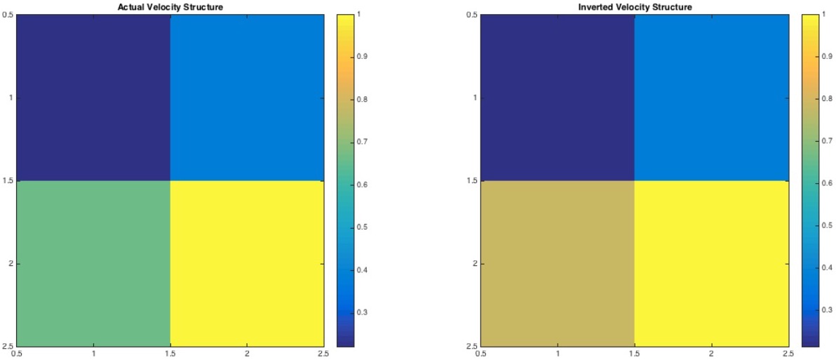
In above figure, we can notice that the cell 3 of the inverted structure is about 10-20% overestimated. We attribute this overestimation due to 20% noise in our data.
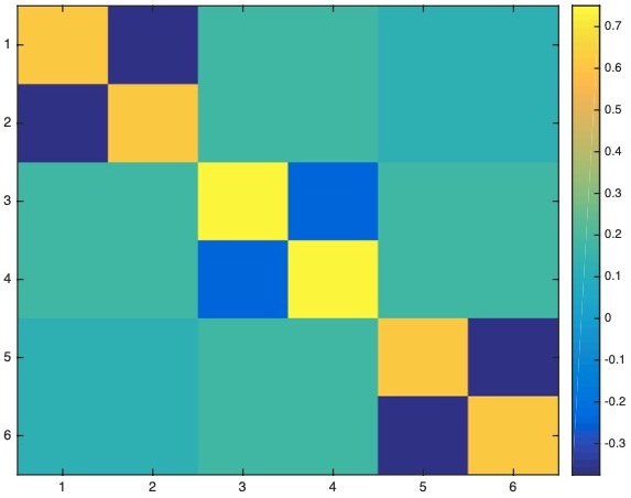
We also estimate the model resolution matrix and the data resolution matrix for this case. The data resolution matrix tells us how well the estimate of the model parameters fits the data and the model resolution matrix tells us how close is the particular estimate of the model parameters is to the true model.
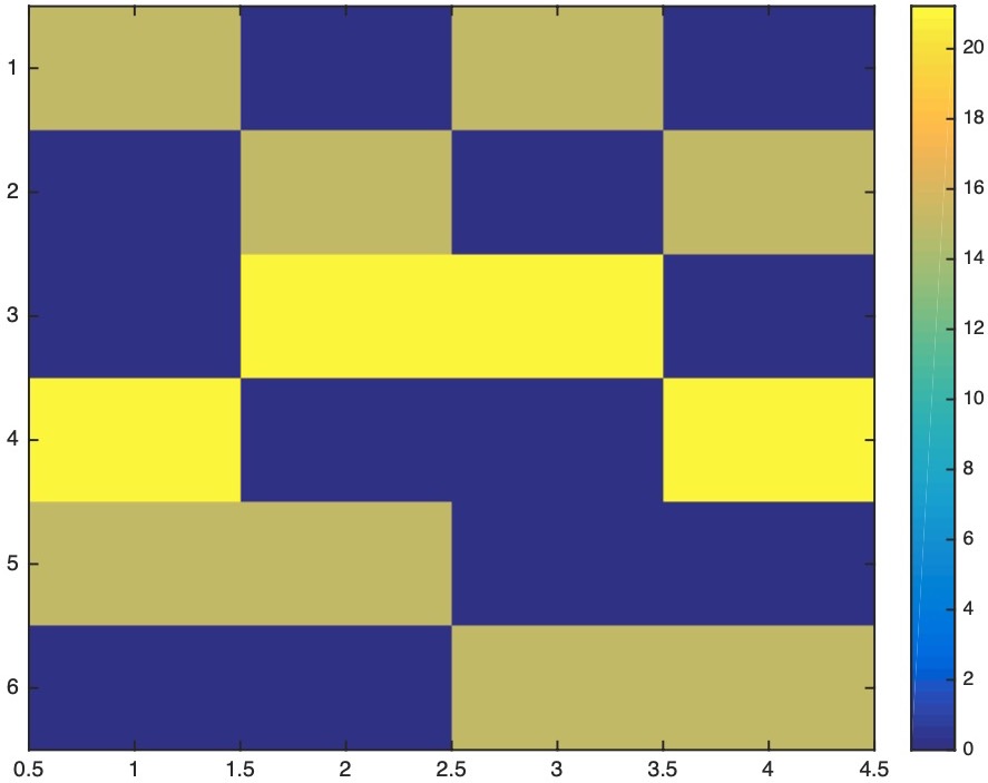
The model resolution matrix is:
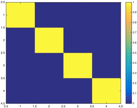
The data resolution matrix is:
\[N = \begin{bmatrix} 0.6250 & -0.3750 & 0.1768 & 0.1768 & 0.1250 & 0.1250 \\ -0.3750 & 0.6250 & 0.1768 & 0.1768 & 0.1250 & 0.1250 \\ 0.1768 & 0.1768 & 0.7500 & -0.2500 & 0.1768 & 0.1768 \\ 0.1768 & 0.1768 & -0.2500 & 0.7500 & 0.1768 & 0.1768 \\ 0.1250 & 0.1250 & 0.1768 & 0.1768 & 0.6250 & -0.3750 \\ 0.1250 & 0.1250 & 0.1768 & 0.1768 & -0.3750 & 0.6250 \end{bmatrix}\]
We estimate the correlation between the two images, and we obtain the correlation to be 0.9883.
To be Continued
Disclaimer of liability
The information provided by the Earth Inversion is made available for educational purposes only.
Whilst we endeavor to keep the information up-to-date and correct. Earth Inversion makes no representations or warranties of any kind, express or implied about the completeness, accuracy, reliability, suitability or availability with respect to the website or the information, products, services or related graphics content on the website for any purpose.
UNDER NO CIRCUMSTANCE SHALL WE HAVE ANY LIABILITY TO YOU FOR ANY LOSS OR DAMAGE OF ANY KIND INCURRED AS A RESULT OF THE USE OF THE SITE OR RELIANCE ON ANY INFORMATION PROVIDED ON THE SITE. ANY RELIANCE YOU PLACED ON SUCH MATERIAL IS THEREFORE STRICTLY AT YOUR OWN RISK.
Leave a comment