Write ASCII data to MSEED file using Obspy (codes included)

Introduction

This post is about reading an ASCII file whose first few lines contain the header information and then the three-component data, and then finally writing it into the Mseed (or SAC) formatted file. I will read the data using the pandas dataframe and then save it into the mseed file using obspy. The header information will also be written into the file.

The ASCII file I used for this post has the following format:

199005111310
 41.49000  130.42000 586.00 24.  12.630  -0.690 -11.940   3.930 -19.500 -12.270   6.80   5.00
HYB
   17.41700   78.55300  510.00000  50.2354 257.5201
3 ZRT
  3601     0.000
    0.000  0.00000000E+00  0.00000000E+00  0.00000000E+00
    1.000  0.00000000E+00  0.00000000E+00  0.00000000E+00
    2.000  0.00000000E+00  0.00000000E+00  0.00000000E+00
    3.000  0.00000000E+00  0.00000000E+00  0.00000000E+00
    4.000  0.00000000E+00  0.00000000E+00  0.00000000E+00
    5.000  0.00000000E+00  0.00000000E+00  0.00000000E+00
    6.000  0.20651668E-07 -0.17604642E-07  0.12335463E-07
    7.000  0.33964160E-07 -0.32352548E-07  0.20258623E-07
    8.000  0.47860410E-07 -0.52818472E-07  0.28573858E-07
    9.000  0.57876023E-07 -0.77652109E-07  0.34789229E-07
   10.000  0.60017179E-07 -0.10427422E-06  0.36822529E-07
   11.000  0.53305714E-07 -0.12976660E-06  0.34412122E-07
   12.000  0.40943924E-07 -0.15182159E-06  0.29569563E-07
   13.000  0.29080783E-07 -0.16921048E-06  0.25574463E-07
   14.000  0.23762603E-07 -0.18157713E-06  0.25058633E-07
   15.000  0.27860320E-07 -0.18878092E-06  0.28412138E-07
   16.000  0.39770686E-07 -0.19026609E-06  0.33568093E-07
   17.000  0.54573346E-07 -0.18492088E-06  0.37330729E-07
   18.000  0.66849783E-07 -0.17162138E-06  0.37408331E-07
   19.000  0.73454726E-07 -0.15025366E-06  0.33857066E-07
   20.000  0.74688101E-07 -0.12267228E-06  0.29021215E-07
   21.000  0.73373968E-07 -0.92971096E-07  0.26016018E-07
   22.000  0.72622052E-07 -0.66704201E-07  0.26728559E-07
   23.000  0.73745417E-07 -0.49206103E-07  0.30615360E-07
   ...

Reading header from the first few lines of the ASCII file

As we can see, the first six lines of the ASCII file contains the header information. The first line is the event id following the origin-time format; the second line is the moment tensor solutions; the third line has the station and event info.

We use the python open method to read that info into the memory to finally write into the mseed file.

import matplotlib.pyplot as plt
import numpy as np
import pandas as pd
import os

dataFileLoc = "OutputWaveforms" #location of the ascii file
dataFileName = "199005111310.HYB.ASC" #ascii file name

dataFile = os.path.join(dataFileLoc, dataFileName)

with open(dataFile, 'r') as ff:
    line = ff.readline()
    eventid=line.strip()
    cnt = 1
    while line:
        print("Line {}: {}".format(cnt, line.strip()))
        line = ff.readline()
        cnt += 1

        if cnt==2:
            mtsol = line.strip()
        elif cnt==3:
            stnName = line.strip()
        elif cnt==4:
            stnLocs = line.strip()
        elif cnt==6:
            dataCounts = line.strip()
        elif cnt>6:
            break

Read the three-component data using the Pandas DataFrame

In the above description of the ASCII data file, we can see that the data is stored in four columns, with the first shows the timestamps, and then the next three columns are the “Z”, “R”, “T”. We can easily read it using the pandas dataframe.

data_df = pd.read_csv(dataFile, skiprows=6, names= ['timestamp', 'Z', 'R', 'T'], sep='\s+', dtype={'Z': np.float64, "R": np.float64, "T": np.float64})

Notice that we have skipped the first six lines as those contain the header info, not the data.

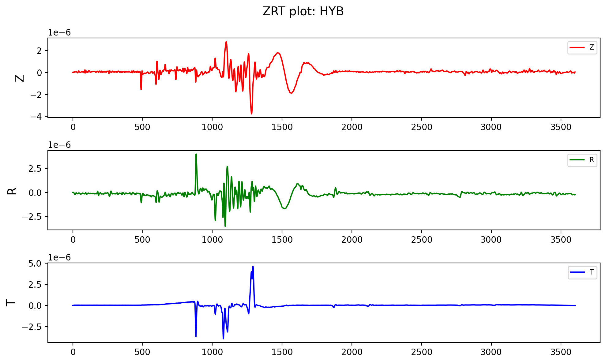
Quick plot of the data using matplotlib

Since we have loaded our data into the pandas dataframe, plotting the data is super simple.

fig, (ax1, ax2, ax3) = plt.subplots(3,1, figsize=(10,6))

ax1.plot(data_df['timestamp'], data_df['Z'], color="r", label="Z")
ax1.set_ylabel("Z", fontsize=14)
ax1.legend(fontsize=8, frameon=True)


plt.suptitle(f"ZRT plot: {stnName}", fontsize=14)


ax2.plot(data_df['timestamp'], data_df['R'], color="g", label="R")
ax2.set_ylabel("R", fontsize=14)
ax2.legend(fontsize=8, frameon=True)


ax3.plot(data_df['timestamp'], data_df['T'], color="b", label="T")
ax3.set_ylabel("T", fontsize=14)
ax3.legend(fontsize=8, frameon=True)

plt.tight_layout()


plt.savefig(os.path.join(dataFileLoc, f"{stnName}-ZRT.png"),
    bbox_inches="tight",
    dpi=200,
)
plt.close('all')

Writing the data to mseed file

To write the data to the mseed file through obspy, we first need to load the data into the obspy object Stream, and then saving and plotting the data is straightforward.

from obspy import Stream, Trace
from obspy.core import UTCDateTime

statsZ = {}
statsZ['network'] = "SYN" #fake network name
statsZ['station'] = stnName
# statsZ['npts'] = dataCounts.split()[0]
statsZ['component'] = 'Z'

## Station location
statsZ['stla'] = stnLocs.split()[0]
statsZ['stlo'] = stnLocs.split()[1]

## Event location
statsZ['evla'] = stnLocs.split()[3]
statsZ['evlo'] = stnLocs.split()[4]
statsZ['evdp'] = stnLocs.split()[2]


statsZ['starttime'] = UTCDateTime(eventid)
trZ = Trace(data=data_df['Z'].values, header = statsZ)

statsR = statsZ
statsR['component'] = 'R'
trR = Trace(data=data_df['R'].values, header = statsR)

statsT = statsZ
statsT['component'] = 'T'
trT = Trace(data=data_df['T'].values, header = statsT)

st = Stream(traces=[trZ, trR, trT])

print(st)

## Write the stream to file
st.write(os.path.join(dataFileLoc, f"{stnName}-ZRT-obspy.mseed"), format="MSEED")

We first used the header info from the ASCII file and wrote that into dictionaries (one for each component), and then we can write the data and the header information using the Trace object of the obspy. Then, we combine the three Trace objects into one stream. Next, we wrote the stream to the mseed file. We can quickly write to any other formats like SAC or others by just changing filename with the different extensions. obspy is smart enough to understand the different formats.

What miniSEED actually keeps. You can attach any custom keys to a Trace’s stats in memory (here stla, stlo, evla, evlo, evdp), but miniSEED does not store them — the format only encodes the SEED identifiers (network/station/location/channel), the timing (starttime, sampling_rate, number of samples), and the data samples. Read the file back and those coordinate fields are gone. To persist station/event coordinates, write SAC instead (its header has stla/stlo/evla/evlo slots — exactly why this workflow keeps them handy) or store the station metadata separately in a StationXML inventory. Also note ObsPy needs the data dtype to be int32, float32, or float64 to write MSEED; the float64 array here writes fine.

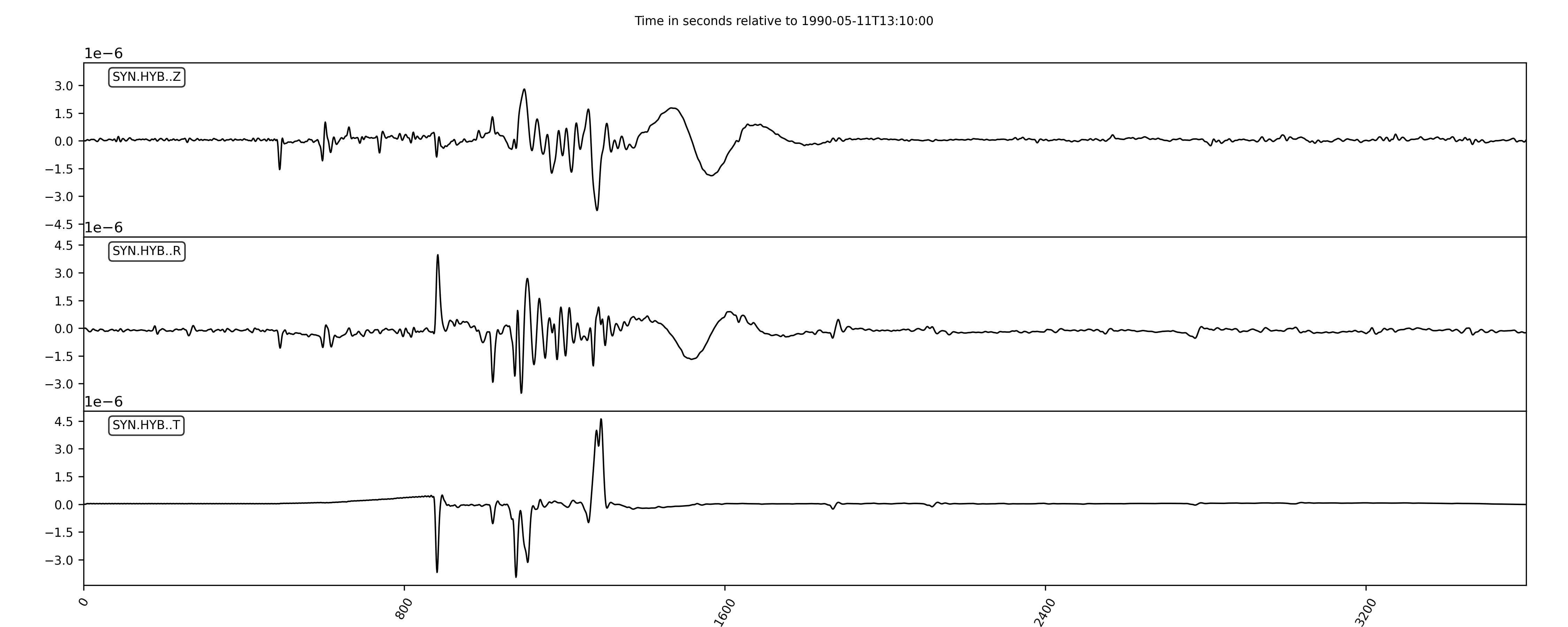
Plot the Obspy stream and save it to the file

Finally, we can also plot the obspy stream using the plot method and then save it into the file.

## Plot the stream
stFig = st.plot(show=False,
        size=(1500,600), number_of_ticks=6,
        type='relative', tick_rotation=60, handle=True,
        linewidth = 1)
plt.savefig(os.path.join(dataFileLoc, f"{stnName}-ZRT-obspy.png"), dpi=300)

Recap

• A raw column of numbers becomes a seismogram only when paired with a Stats header (network, station, component, starttime, sampling_rate) inside a Trace.
• Read the ASCII header lines with plain open()/readline(), load the numeric columns with pandas, then build one Trace per component and group them in a Stream.
• st.write(..., format="MSEED") saves the Stream; swap the format string (e.g. "SAC") to write other formats from the same object.
• miniSEED keeps only the SEED id, timing, and samples — for station/event coordinates use SAC or a StationXML inventory.
• MSEED needs an int32/float32/float64 data array; the float64 array from pandas writes without any casting.

Where to go next

• Getting started with ObsPy for seismologists — the Trace/Stream/Stats basics in depth.
• Plotting a record section with ObsPy — visualize many traces together once they carry distance metadata.
• Concatenating daily seismic traces and plotting a spectrogram — more ObsPy waveform handling.
• How to start using pandas for Earth data analysis — the dataframe reading used here.

Complete Script