Least-Squares Method in Geosciences (codes included)
Least-squares method is a popular approach in geophysical inversion to estimate the parameters of a postulated Earth model from given observations. This method estimates the solution of an inverse problem by finding the best model parameters that minimizes the measure of length of prediction error, the Euclidean length
Introduction
Least-squares method is a popular approach in geophysical inversion to estimate the parameters of a postulated Earth model from given observations. This method estimates the solution of an inverse problem by finding the best model parameters that minimizes the measure of length of prediction error, the Euclidean length \( d^{obs}- d^{pre} \) (Menke 2018). There are several titles available that discusses this approach in details but since we regularly use this method for several applications, it is important to introduce this method in brief.
A geophysical model can be linear or non-linear function of model parameters. However, most of the complex geophysical models tend to be non-linear in nature. Let us introduce the least-squares concept for the earthquake location problem in the homogenous medium. Earthquake location problem are inherently non-linear.
Least-Squares Problem: Earthquake location in homogeneous medium
I take the simplest case of locating the earthquake in a medium with uniform velocity of v. Since the medium has uniform velocity, the ray paths connecting the source and receiver are straight lines. In real scenario, this is true only in the case of the source and receiver to be very close to each other. The arrival times of the seismic waves at several seismic stations (\( x_i, y_i, z_i \)) from an earthquake occurring at time \( t \), at location (\( x,y,z \)) can be expressed as:
\begin{equation} \label{eq:square} \begin{split} d_i &=[(x-x_i )^2+(y-y_i )^2+(z-z_i )^2 ]^(1/2)/v+t \end{split} \end{equation}
where \( d_i \) is the arrival time data at station \( i \). The parameters \( x_i, y_i, z_i, d_i \) are known and the unknowns are the location \( (x,y,z) \) , the velocity \( v \) and the origin time \( t \), of the earthquake. Here, we can notice that the model is non-linear. We can assume that the station is at the surface, hence \( z_i= 0 \).
To solve this problem, I begin with the starting model vector \( m^0= (x_0,y_0,z_0,v_0,t_0 )\) . This starting model vector is chosen based on the educated guess so that the solution is close to what we seek. We then wish to improve the model parameters iteratively such that the predicted arrival time \( d_i^{pre} \) at each iteration is closer to the observed arrival time \( d_i \).
One way to achieve the solution to this non-linear problem is by linearizing it using the Taylor series expansion. We form the matrix of partial derivatives \( G_ij \) of the elements of the arrival time data with respect to the model parameters.
\begin{equation}
\label{eq:eq_partials1}
\begin{split}
G_{i1} &=(\partial d_i)/\partial x
&= (x-x_i ) [(x-x_i )^2+(y-y_i )^2+z^2 ]^(-1/2)/v
\end{split}
\end{equation}
\begin{equation}
\label{eq:eq_partials2}
\begin{split}
G_{i2} &=(\partial d_i)/\partial y
&= (y-y_i ) [(x-x_i )^2+(y-y_i )^2+z^2 ]^(-1/2)/v
\end{split}
\end{equation}
\begin{equation}
\label{eq:eq_partials3}
\begin{split}
G_{i3} &=(\partial d_i)/\partial z
&= z [(x-x_i )^2+(y-y_i )^2+z^2 ]^(-1/2)/v
\end{split}
\end{equation}
\begin{equation}
\label{eq:eq_partials4}
\begin{split}
G_{i4} &=(\partial d_i)/\partial v
&= -[(x-x_i )^2+(y-y_i )^2+z^2 ]^(1/2)/v^2
\end{split}
\end{equation}
\begin{equation}
\label{eq:eq_partials5}
\begin{split}
G_{i5} &=(\partial d_i)/\partial t
&= \partial t/\partial t = 1
\end{split}
\end{equation}
We seek to minimize the difference between the observed and predicted arrival time data, \( \Delta d_i \) . This can be written as
\begin{equation}
\begin{split}
d_i-d_i^0 &= \sum_j[G_ij m_j ] - \sum_j[G_ij [m_j]^0 ]
\Delta d_i &= \sum_j[G_ij \Delta m_j ]
\end{split}
\end{equation}
\begin{equation} \begin{split} \chi^2 &= \sum_i(\Delta d_i- \sum_j[G_ij \Delta m_j ])^2 \end{split} \end{equation}
This is the least-squares objective function which can be solved for the best model parameters for the earthquake location. Here we have also assumed that the arrival time data do not have any errors. In reality, the observations always contain some errors due to variety of reasons such as reading errors, misidentification of first arrivals etc.
We seek to minimize the value of \( \chi^2 \) for the best solution of \( \Delta m_j \) . Traditionally, this can be done by setting the partial derivative of above equation to zero. This gives us the solution of the form (also commonly known as generalized inverse):
\begin{equation} \label{eq:eq2} \Delta m = (G^T G)^{-1} G^T \Delta d \end{equation}
Hypothetical earthquake location problem
Let us consider a hypothetical example of the earthquake location problem with six stations. The arbitrarily chosen location of the stations are listed in Table 1. Let us consider the earthquake location to be (2,2,-2) and the velocity of the homogeneous medium to be 6 unit/s. This is an over-determined problem as the number of equations is greater than the number of solutions. When the number of non-trivial equations in an inverse problem is more than the number of solutions, it is called overdetermined problem and underdetermined otherwise. In reality, we seek the complex geophysical problems to be overdetermined because as we need to deal with the errors and noise. More number of equations (or data) improve the reliability of the solution.
Table 1: Hypothetical earthquake location problem: locations of stations and the corresponding arrival time of seismic wave.
| Station x-position | Station y-position | Station z-position | Arrival time (with 5% error) |
|---|---|---|---|
| 0.20 | -0.37 | 0 | 0.63 |
| 0.86 | 2.35 | 0 | 0.41 |
| 0.41 | 2.78 | 0 | 0.47 |
| 0.18 | -0.70 | 0 | 0.67 |
| -0.31 | 1.75 | 0 | 0.54 |
| 0.58 | 0.17 | 0 | 0.53 |
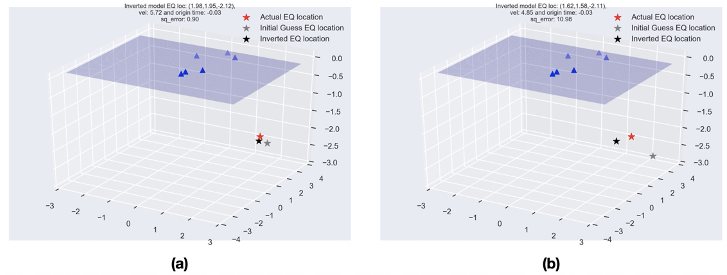
Figure 1: Hypothetical earthquake location solution using generalized inverse.
The actual earthquake location is (2,2,-2), velocity of the homogeneous medium is 6 unit/s, and the actual origin time is 0s. (a) The error in initial guess is 10% of the actual model parameters (b) The error in initial guess is 30% of the actual model parameters.
import random

import matplotlib.pyplot as plt
import numpy as np
import pandas as pd
from matplotlib import cm
from mpl_toolkits.mplot3d import Axes3D
from numpy.linalg import inv

np.random.seed(0)

plt.style.use('seaborn')
error = 0.10 #10 percent


minx, maxx = -2, 2
miny, maxy = -3, 3
# stn_locs = [[-2,3,0],[1,3,0],[-2,-1,0],[0,-3,0],[2,-2,0]]
numstations = 30
stn_locs=[]
xvals = minx+(maxx-minx)*np.random.rand(numstations)
yvals = miny+(maxy-miny)*np.random.rand(numstations)

for num in range(numstations):
    stn_locs.append([xvals[num],yvals[num],0])

eq_loc = [2,2,-2]
vel = 6 #kmps
origintime = 0

def calc_arrival_time(eq_loc, stnx, stny, stnz, vel, origintime):
    eqx, eqy, eqz = eq_loc
    dist = np.sqrt((eqx - stnx)**2 + (eqy - stny)**2 + (eqz - stnz)**2)
    arr = dist/vel + origintime
    return arr

def G_matrix_cols(eq_loc, stnx, stny, stnz, vel, origintime):
    eqx, eqy, eqz = eq_loc
    G_col1 = (eqx-stnx)/vel * ((eqx - stnx)**2 + (eqy - stny)**2 + (eqz - stnz)**2)**(-1/2)
    G_col2 = (eqy-stny)/vel * ((eqx - stnx)**2 + (eqy - stny)**2 + (eqz - stnz)**2)**(-1/2)
    G_col3 = (eqz-stnz)/vel * ((eqx - stnx)**2 + (eqy - stny)**2 + (eqz - stnz)**2)**(-1/2)
    G_col4 = -1/vel**2 * ((eqx - stnx)**2 + (eqy - stny)**2 + (eqz - stnz)**2)**(1/2)
    G_col5 = 1
    return [G_col1,G_col2,G_col3,G_col4,G_col5]


eq_initial_guess = [eq_loc[0]+error*eq_loc[0],eq_loc[1]+error*eq_loc[1],eq_loc[2]+error*eq_loc[2]]
m_intial = [eq_initial_guess[0],eq_initial_guess[1],eq_initial_guess[2],vel+error*vel,origintime+error*origintime]


G_matrix = []
d_obs = []
d_pre = []
noise_level_data = 0.1
# noise_level_data = 0.001
for stnx, stny, stnz in stn_locs:
    # print("{:.2f} {:.2f} {:d}".format(stnx, stny, stnz))
    arr = calc_arrival_time(eq_loc, stnx, stny, stnz, vel, origintime)
    G_matrix.append(G_matrix_cols(eq_initial_guess, stnx, stny, stnz, m_intial[3], m_intial[4]))
    sign = np.random.choice([-1,1])
    d_obs.append(arr+sign*noise_level_data*arr)
    print("Arrival time at ({},{},{}) is {}".format(stnx, stny, stnz, arr+sign*noise_level_data*arr))
    # print("{:.2f}".format(arr+0.05*arr))
    d_pre.append(calc_arrival_time(eq_initial_guess, stnx, stny, stnz, m_intial[3], m_intial[4]))

d_obs = np.array(d_obs)
d_pre = np.array(d_pre)
G_matrix = np.array(G_matrix)


delm = inv(np.transpose(G_matrix).dot(G_matrix)).dot(np.transpose(G_matrix)).dot(d_obs-d_pre)
inv_model = m_intial+delm


print("Actual model EQ loc: ({:.2f},{:.2f},{:.2f}), vel: {:.2f} and origin time: {:.2f}".format(eq_loc[0],eq_loc[1],eq_loc[2],vel,origintime))
print("Initial model EQ loc: ({:.2f},{:.2f},{:.2f}), vel: {:.2f} and origin time: {:.2f}".format(m_intial[0],m_intial[1],m_intial[2],m_intial[3],m_intial[4]))
print("Inverted model EQ loc: ({:.2f},{:.2f},{:.2f}), vel: {:.2f} and origin time: {:.2f}".format(inv_model[0],inv_model[1],inv_model[2],inv_model[3],inv_model[4]))

squared_error = np.sum((inv_model-m_intial)**2)


## to create the surface
X = np.linspace(-3, 3, 200)
Y = np.linspace(-3, 3, 200)
X, Y = np.meshgrid(X, Y)
Z = (X**2 + Y**2)*0

fig = plt.figure()
ax = plt.axes(projection='3d')
# plot stations
ax.scatter([x[0] for x in stn_locs],[x[1] for x in stn_locs],[x[2] for x in stn_locs],c='b',marker='^',s=50)
# plot surface
surf = ax.plot_surface(X, Y, Z, rstride=1, cstride=1, cmap=cm.jet,linewidth=0, antialiased=False,alpha=0.1)
# plot actual EQ
ax.scatter(eq_loc[0],eq_loc[1],eq_loc[2],c='r',marker='*',s=100,label='Actual EQ location')
ax.scatter(eq_initial_guess[0],eq_initial_guess[1],eq_initial_guess[2],c='gray',marker='*',s=100,label='Initial Guess EQ location')
ax.scatter(inv_model[0],inv_model[1],inv_model[2],c='k',marker='*',s=100,label='Inverted EQ location')
plt.title("Inverted model EQ loc: ({:.2f},{:.2f},{:.2f}),\nvel: {:.2f} and origin time: {:.2f}\nsq_error: {:.2f}".format(inv_model[0],inv_model[1],inv_model[2],inv_model[3],inv_model[4],squared_error),fontsize=8)
ax.set_xlim([-3,3])
ax.set_ylim([-4,4])
ax.set_zlim(-3,0.1)
plt.legend()

plt.savefig('Earthquake_loc_{:.0f}stn_{:.0f}percent_error.png'.format(numstations,error*100),bbox_inches='tight',dpi=300)
# plt.savefig('Earthquake_loc_5stn_30percent_error.png',bbox_inches='tight',dpi=300)
plt.close('all')
Source Code:
![]()
The six stations and the actual earthquake location of \( (2,2,-2) \) is used to generate arrival time data at each station (Table 1). I added 0.1% random error in arrival time data. I estimated the model parameters using Equation \eqref{eq:eq2} assuming some arbitrary initial guess with 10% and 30% difference from the actual model parameters (see Figure 1). The squared error in the estimation of model parameters in the two cases is 0.90 and 10.98. This approach to find the minimum of the least-squares problem depends heavily on the initial model parameters. Also, 6 stations are not sufficient to invert for the earthquake location within a reasonable uncertainty as the real data most often is contaminated by more noise. When I inverted for the same 10% and 30% error in the initial guess and 6 stations for higher noise level of just 1%, the squared error in the two cases becomes 507.6 and 1250.25, respectively. However, when I took 30 stations for the same level of noise in the arrival time observations, the squared error reduced to 18.33 and 55.22, respectively.
In this hypothetical earthquake location problem, we used the Equation \eqref{eq:eq2}, and inverted directly. However, for larger problems, the inversion is computationally intensive or impossible and hence this approach is prohibitive. In such cases, it is preferred to use the iterative matrix solver such as biconjugate gradient algorithm (Barrett et. al., 1994).
Local vs Global Optimization Problem
The common geophysical problems often have the multimodal objective function for the least-squares problem with many local minima which are not global minima (Figure 2). Initial guess of the model parameters near the local minima tend to converge to local minimum of the least-squares objective function. Numerical algorithms such as steepest descent, Newton’s method, Quasi-Newton method, conjugate gradient method etc. (Kutz, 2013) tends to get trapped in the local minima if the initial parameters are not wisely chosen. That is because they use the search for the direction of optimal value and move towards it iteratively.
In complex problems with many local minima, it is imperative to look for some global search methods. One of the most common approach in such cases it to adapt grid method which is an exact search method. It looks for all the possible solutions in the parameter space and then resolve the global minima. This approach is computationally intensive for many parameters’ problems (curse of dimensionality). It’s computational cost also has trade-off with the resolution of the final solution. Although this method can be improved using constrains of the search bounds or removing infeasible points and adopting sparse grids. Other global search method includes Monte Carlo, Simulated Annealing, Genetic Algorithms, etc (Menke, 2018). These methods do not compute the objective function for all the possible solutions but follow set of rules to cleverly sample the parameter space in order to simulate the working of the system and find the optimal solution.
import numpy as np
import matplotlib.pyplot as plt
plt.style.use('seaborn')


## Example 1
x = np.linspace(-3,3,100)
obj_fun = np.cos(14.5 * x - 0.3) + x*(x + 0.2) + 1.01

fig, ax = plt.subplots(1,1,figsize=(10,6))
ax.plot(x,obj_fun)
ax.axvline(x = x[np.argmin(obj_fun)],color='r',ls='--')
ax.set_ylabel(r'$f(x)$')
ax.set_xlabel(r'$x$')
plt.savefig('local_global_objective_function.png',dpi=300,bbox_inches='tight')
plt.close('all')


## Example 2 Surface plot
from matplotlib import cm
from mpl_toolkits.mplot3d import Axes3D


x2 = np.linspace(-6,6,100)
y2 = np.linspace(-6,6,100)
X,Y = np.meshgrid(x2,y2)

obj_fun2 = ((X+0.5)**4 - 30*X**2- 20*X + (Y+0.5)**4 - 30*Y**2- 20*Y)/100

fig = plt.figure(figsize=(5,5))
ax = fig.gca(projection='3d')
# Plot the surface.
surf = ax.plot_surface(X, Y, obj_fun2, cmap=cm.jet,linewidth=0, antialiased=False)
ax.set_ylabel(r'$x$')
ax.set_xlabel(r'$y$')
plt.savefig('local_global_objective_function3D.png',dpi=300,bbox_inches='tight')
plt.close('all')


## Example 2 contour plot


fig, ax = plt.subplots(1,1,figsize=(6,5))
cp = ax.contourf(X, Y, obj_fun2, 20, cmap='jet')
plt.colorbar(cp)
# ax.clabel(cp, inline=True, fontsize=10)

ax.set_ylabel(r'$y$')
ax.set_xlabel(r'$x$')
plt.savefig('local_global_objective_function_contour.png',dpi=300,bbox_inches='tight')
plt.close('all')
Source Code:
![]()
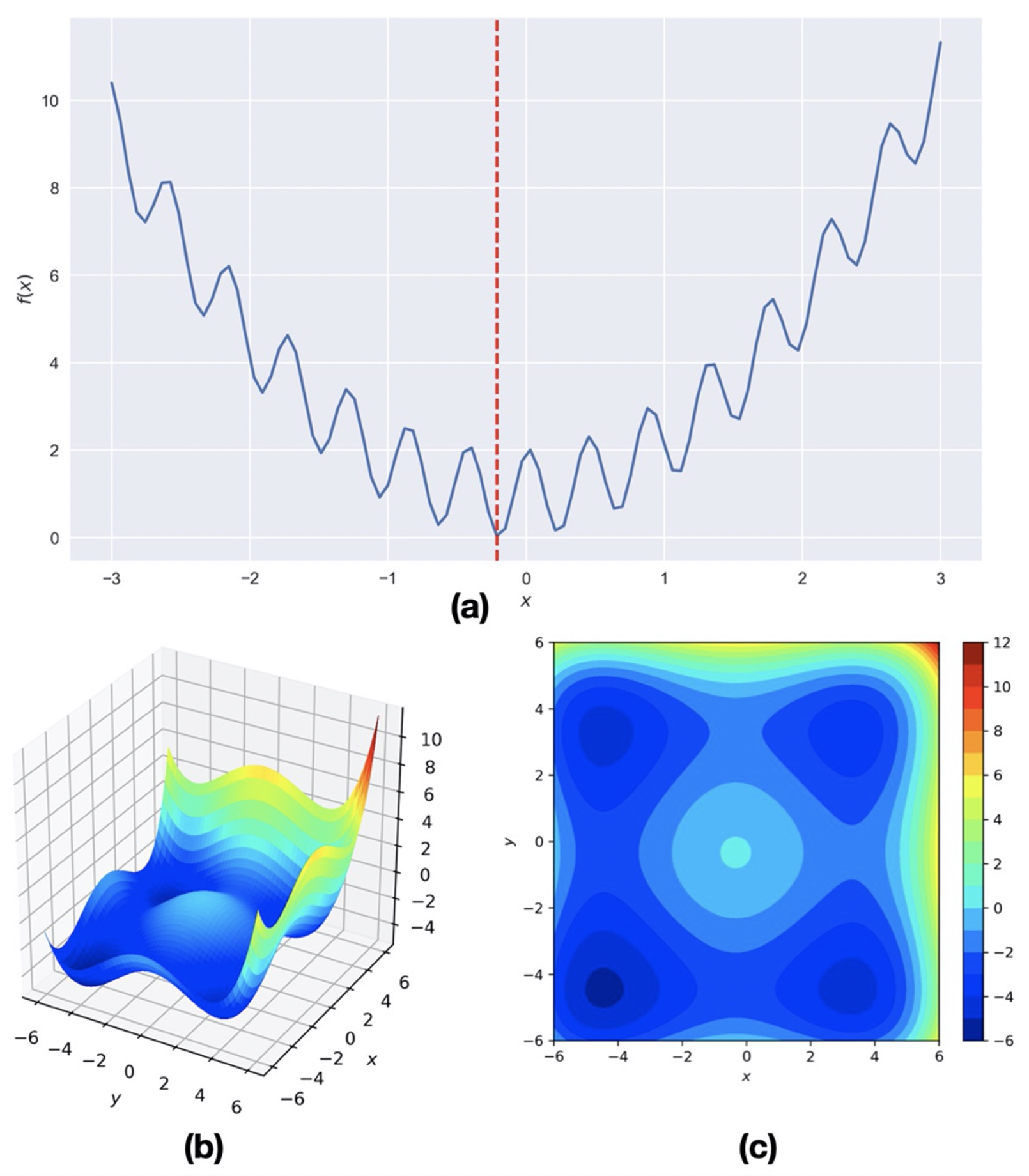
Figure 2: Hypothetical objective functions with global and local minima.
(a) The objective function is \(cos(14.5x-0.3)+x(x+0.2)+1.01 \) . There are many local minima. The global minimum is at -0.2. Local search method tends to converse to local minima with the initial model parameter close to it. (b-c) Surface and contour plot of \([\sum_(i=1)^2[(x_i+ 0.5)^4-30 x_i^2- 20 x_i ]]/100 \) .
Disclaimer of liability
The information provided by the Earth Inversion is made available for educational purposes only.
Whilst we endeavor to keep the information up-to-date and correct. Earth Inversion makes no representations or warranties of any kind, express or implied about the completeness, accuracy, reliability, suitability or availability with respect to the website or the information, products, services or related graphics content on the website for any purpose.
UNDER NO CIRCUMSTANCE SHALL WE HAVE ANY LIABILITY TO YOU FOR ANY LOSS OR DAMAGE OF ANY KIND INCURRED AS A RESULT OF THE USE OF THE SITE OR RELIANCE ON ANY INFORMATION PROVIDED ON THE SITE. ANY RELIANCE YOU PLACED ON SUCH MATERIAL IS THEREFORE STRICTLY AT YOUR OWN RISK.