Visualizing power spectral density using Obspy in Python (codes included)
For details, visit Visualizing Probabilistic Power Spectral Densities.
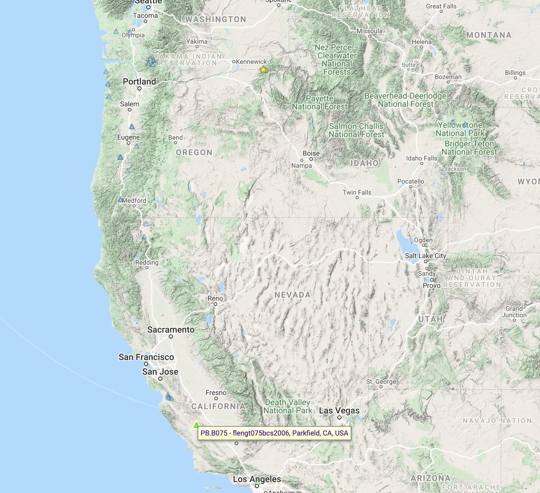
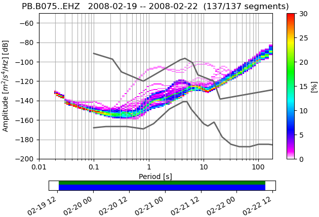
Key idea — a PPSD summarizes hours of noise into one probability picture. An ordinary power spectral density (PSD) turns one window of a seismogram into power-versus-frequency. A probabilistic PSD goes further: it chops a long record (here 3 days of station PB.B075) into many overlapping windows, computes a PSD for each, and bins them all into a 2-D histogram of power (dB) versus period. The result shows, at every period, how often each noise level occurs — so persistent site noise, the microseism peaks, and intermittent glitches all separate out. ObsPy’s PPSD class does the whole pipeline and frames the plot with Peterson’s New High/Low Noise Models (NHNM/NLNM) as reference bounds.
Data source note (2026): the waveforms and station response are pulled from the IRIS FDSN web services via Client('IRIS'). IRIS merged with UNAVCO in 2023 to form EarthScope; the data services continue and Client("IRIS") still resolves as an alias, so this code runs unchanged.
Contents
- Import necessary libraries
- Download stream using Obspy
- Add data to the ppsd estimate
- Visualization using Obspy
- Output Figures
- References
Import necessary libraries
from obspy.io.xseed import Parser
from obspy.signal import PPSD
from obspy.clients.fdsn import Client
from obspy import UTCDateTime, read_inventory, read
import os, glob
import matplotlib.pyplot as plt
from obspy.imaging.cm import pqlx
import warnings
warnings.filterwarnings('ignore')
Download stream using Obspy
## Downloading inventory
net = 'PB'
sta = 'B075'
loc='*'
chan = 'EH*'
filename_prefix = f"{net}_{sta}"
mseedfiles = glob.glob(filename_prefix+".mseed")
xmlfiles = glob.glob(filename_prefix+'_stations.xml')

if not len(mseedfiles) or not len(xmlfiles):
    print("--> Missing mseed / station xml file, downloading...")
    time = UTCDateTime('2008-02-19T13:30:00')
    wf_starttime = time - 60*60
    wf_endtime = time + 3 * 24 * 60 * 60 #3 days of data (requires atleast 1 hour)

    client = Client('IRIS')

    st = client.get_waveforms(net, sta, loc, chan, wf_starttime, wf_endtime)
    st.write(filename_prefix+".mseed", format="MSEED")
    inventory = client.get_stations(starttime=wf_starttime, endtime=wf_endtime,network=net, station=sta, channel=chan, level='response', location=loc)
    inventory.write(filename_prefix+'_stations.xml', 'STATIONXML')
else:
    st = read(filename_prefix+".mseed")
    inventory = read_inventory(filename_prefix+'_stations.xml')
Add data to the ppsd estimate
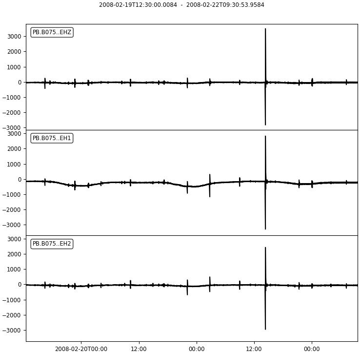
tr = st.select(channel="EHZ")[0]
print(st)
st.plot(outfile=filename_prefix+"traces.png",show=False)
ppsd = PPSD(tr.stats, metadata=inventory)
add_status = ppsd.add(st) #add data (either trace or stream objects) to the ppsd estimate
Visualization using Obspy
if add_status:
    print(ppsd)
    print(ppsd.times_processed[:2]) #check what time ranges are represented in the ppsd estimate
    print("Number of psd segments:", len(ppsd.times_processed))
    ppsd.plot(filename_prefix+"-ppsd.png",cmap=pqlx) #colormap used by PQLX / [McNamara2004]
    plt.close('all')
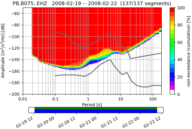
    ppsd.plot(filename_prefix+"-ppsd_cumulative.png",cumulative=True,cmap=pqlx) #cumulative version of the histogram
    plt.close('all')
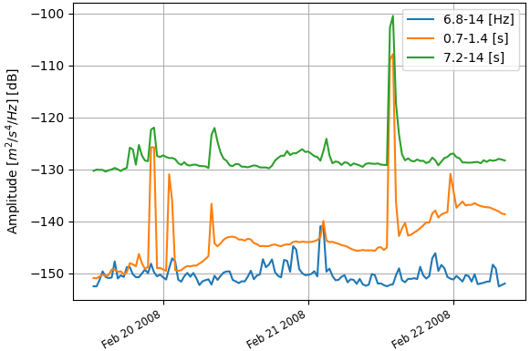
    ppsd.plot_temporal(period=[0.1, 1.0, 10], filename=filename_prefix+"-ppsd_temporal_plot.png") #The central period closest to the specified period is selected
    plt.close('all')
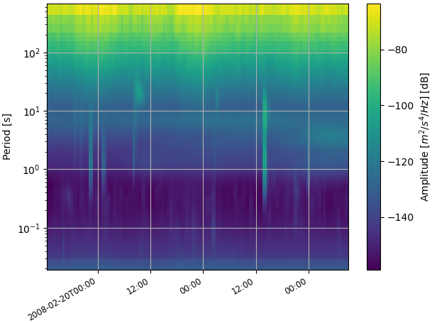
    ppsd.plot_spectrogram(filename=filename_prefix+"-spectrogram.png", show=False)
Output Figures
Quick check: What makes a probabilistic PSD (PPSD) different from a single PSD of the whole record?
- It uses a logarithmic frequency axis instead of a linear one
- It removes the instrument response, which a plain PSD cannot
- It splits the record into many windows and bins their PSDs into a 2-D histogram, showing how often each power level occurs at each period
- It only works on exactly three days of data
Recap
- A PPSD turns a long noise record into a 2-D probability histogram of power (dB) vs. period — revealing the distribution of noise, not just one average spectrum.
- ObsPy’s workflow: download waveforms + response (
Client.get_waveforms/get_stations), buildPPSD(tr.stats, metadata=inventory), then.add(stream)to accumulate windows. - Visualize four ways:
.plot(the histogram, here with thepqlxcolormap),.plot(cumulative=True),.plot_temporal(period=[...])for how power at chosen periods drifts over time, and.plot_spectrogram(). - The
pqlxcolormap and the NHNM/NLNM reference curves come from McNamara & Buland (2004) — the noise-model framework the PPSD was designed around. - Metadata matters: modern ObsPy reads station response from StationXML via
read_inventory; the legacyobspy.io.xseed.Parser(dataless SEED) still works but StationXML is the current path.
Where to go next
- Getting started with ObsPy — Part I — downloading and handling the waveform data feeding this PPSD.
- Signal denoising using the Fast Fourier Transform — the frequency-domain foundations behind a power spectrum.
- ObsPy PPSD tutorial — the official reference for every
PPSDoption.
References
- McNamara, D. E., & Buland, R. P. (2004). Ambient Noise Levels in the Continental United States. Bulletin of the Seismological Society of America, 94(4), 1517–1527.
- McNamara, D. E., & Boaz, R. I. (2005). Seismic Noise Analysis System Using Power Spectral Density Probability Density Functions: A Stand-Alone Software Package. U.S. Geological Survey Open-File Report 2005-1438.
This post was last modified at 2026-10-06 20:47.
Disclaimer of liability
The information provided by the Earth Inversion is made available for educational purposes only.
Whilst we endeavor to keep the information up-to-date and correct. Earth Inversion makes no representations or warranties of any kind, express or implied about the completeness, accuracy, reliability, suitability or availability with respect to the website or the information, products, services or related graphics content on the website for any purpose.
UNDER NO CIRCUMSTANCE SHALL WE HAVE ANY LIABILITY TO YOU FOR ANY LOSS OR DAMAGE OF ANY KIND INCURRED AS A RESULT OF THE USE OF THE SITE OR RELIANCE ON ANY INFORMATION PROVIDED ON THE SITE. ANY RELIANCE YOU PLACED ON SUCH MATERIAL IS THEREFORE STRICTLY AT YOUR OWN RISK.
Leave a comment