Signal denoising using Fourier Analysis in Python (codes included)
Fourier analysis is based on the idea that any time series can be decomposed into a sum of integral of harmonic waves of different frequencies. Hence, theoretically, we can employ a number of harmonic waves to generate any signal.
Key idea — denoise by editing the frequency spectrum, not the time series. The FFT rewrites your signal as a sum of frequencies. The trick this post uses: real signal concentrates into a few high-power peaks, while random noise is spread thinly across all frequencies as a low noise floor. So you transform to the frequency domain, zero out every component whose power is below a threshold, and inverse-transform back — keeping the peaks, dropping the noise. The one assumption is that signal and noise overlap in time but separate in frequency.
The Fourier series for an arbitrary function of time $f(t)$ defined over the interval $-T/2 < t < T/2$ is
\[f(t) = a_0 + \sum_{n=1}^{\infty} a_n \cos\left(\frac{2n\pi t}{T}\right) + \sum_{n=1}^{\infty} b_n \sin\left(\frac{2n\pi t}{T}\right)\]In the above equation, we can see that the $\sin(\frac{2n\pi t}{T})$ and $\cos(\frac{2n\pi t}{T})$ are periodic with period $T/n$ or frequency $n/T$. Here, the larger values of $n$ correspond to shorter periods, or higher frequencies.
In this post, we will use Fourier analysis to filter with the assumption that noise is overlapping the signals in the time domain but are not so overlapping in the frequency domain.
Import libraries, create a signal, and add noise
import pandas as pd
import os, sys
import numpy as np
import matplotlib.pyplot as plt
plt.rcParams['figure.figsize'] = [10,6]
plt.rcParams.update({'font.size': 18})
plt.style.use('seaborn')
## Create synthetic signal
dt = 0.001
t = np.arange(0, 1, dt)
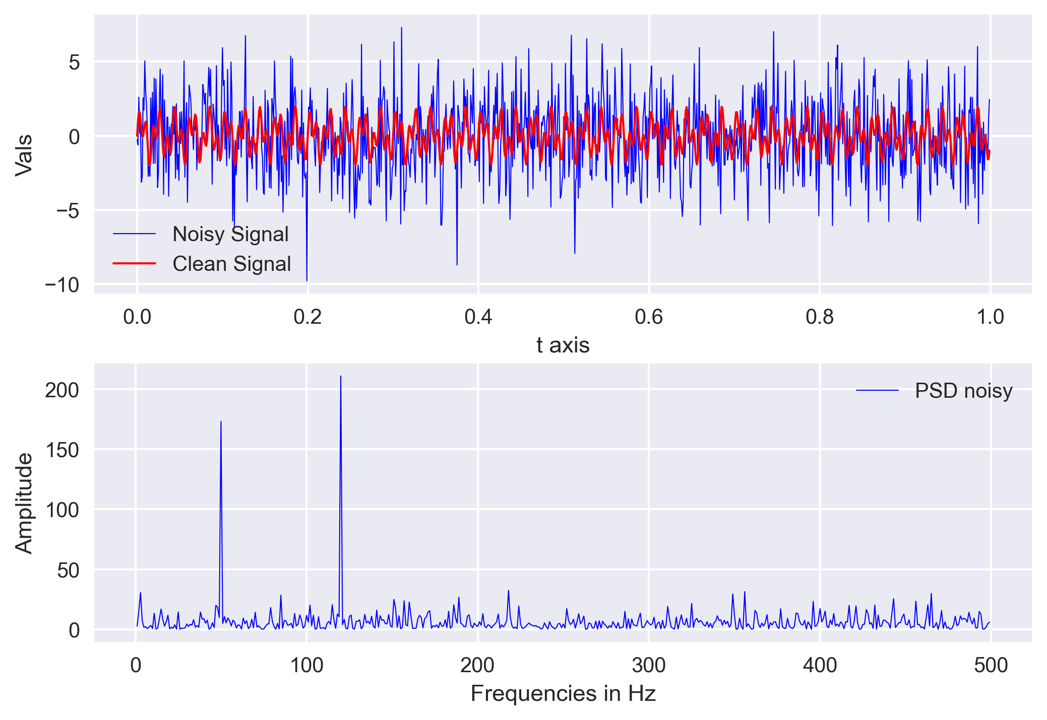
signal = np.sin(2*np.pi*50*t) + np.sin(2*np.pi*120*t) #composite signal
signal_clean = signal #copy for later comparison
signal = signal + 2.5 * np.random.randn(len(t))
minsignal, maxsignal = signal.min(), signal.max()
We created our signal by summing two sine functions different frequencies (50Hz and 120Hz). Then we created an array of random noise and stacked that noise onto the signal.
Matplotlib note: plt.style.use('seaborn') (used in every code block here) was removed in Matplotlib 3.8 — use plt.style.use('seaborn-v0_8') on a current install. The numpy.fft and ObsPy calls are unchanged.
Perform Fast Fourier Transform
## Compute Fourier Transform
n = len(t)
fhat = np.fft.fft(signal, n) #computes the fft
psd = fhat * np.conj(fhat)/n
freq = (1/(dt*n)) * np.arange(n) #frequency array
idxs_half = np.arange(1, np.floor(n/2), dtype=np.int32) #first half index
Numpy’s fft.fft function returns the one-dimensional discrete Fourier Transform with the efficient Fast Fourier Transform (FFT) algorithm. The output of the function is complex and we multiplied it with its conjugate to obtain the power spectrum of the noisy signal. We created the array of frequencies using the sampling interval (dt) and the number of samples (n).
Filter out the noise
In the above plot, we can see that the two frequecies from our original signal is standing out. Now, we can create a filter that can remove all frequencies with amplitude less than our threshold.
## Filter out noise
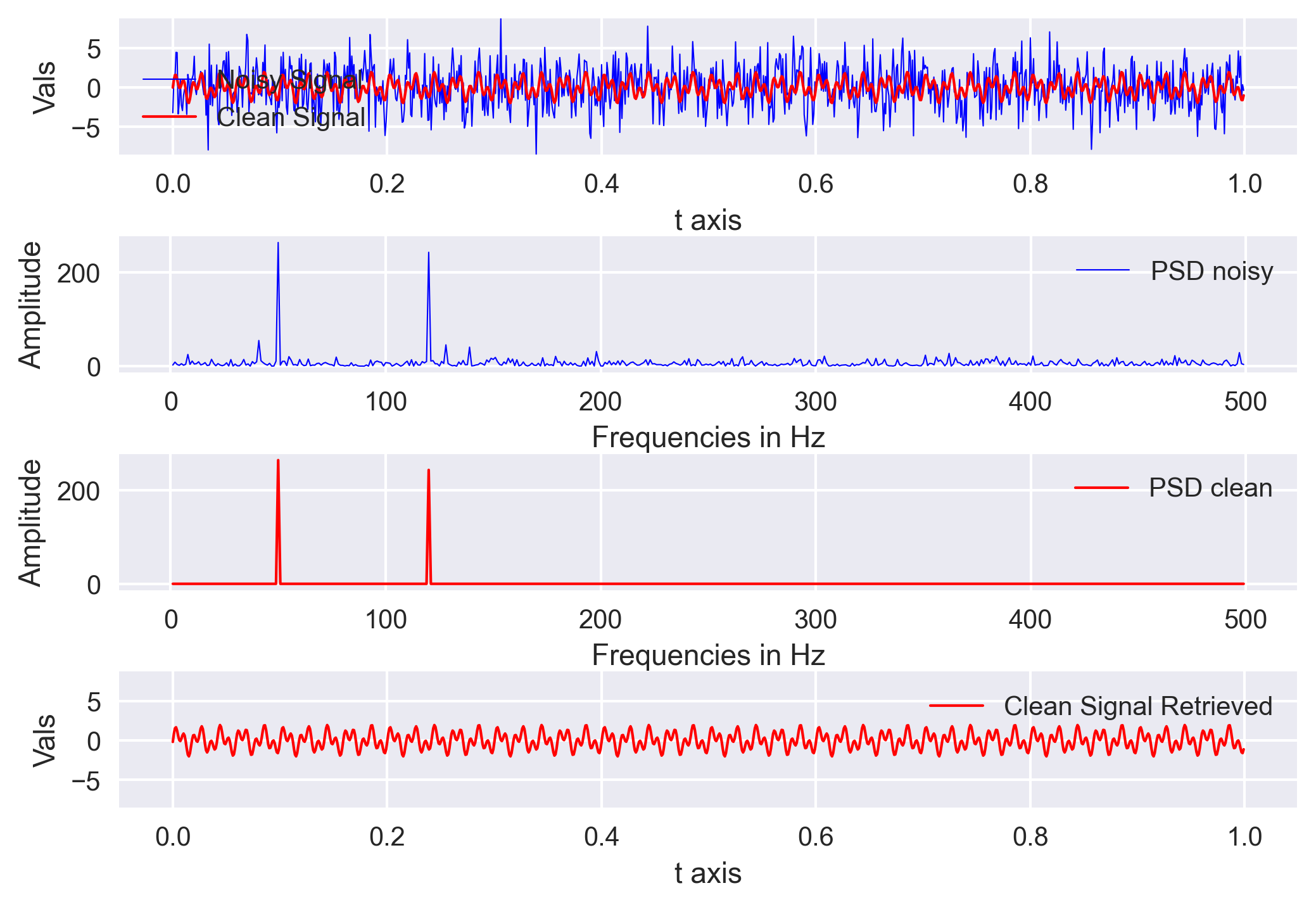
threshold = 100
psd_idxs = psd > threshold #array of 0 and 1
psd_clean = psd * psd_idxs #zero out all the unnecessary powers
fhat_clean = psd_idxs * fhat #used to retrieve the signal
signal_filtered = np.fft.ifft(fhat_clean) #inverse fourier transform
Read those four lines against the diagram: psd > threshold builds a mask (1 where the power beats the threshold, 0 elsewhere), multiplying it into fhat zeros out the sub-threshold frequencies, and np.fft.ifft transforms the surviving peaks back to a clean time series.
Quick check: Why is the threshold applied to psd (the power) rather than directly to the raw signal amplitudes in time?
Visualization the results
## Visualization
fig, ax = plt.subplots(4,1)
ax[0].plot(t, signal, color='b', lw=0.5, label='Noisy Signal')
ax[0].plot(t, signal_clean, color='r', lw=1, label='Clean Signal')
ax[0].set_ylim([minsignal, maxsignal])
ax[0].set_xlabel('t axis')
ax[0].set_ylabel('Vals')
ax[0].legend()

ax[1].plot(freq[idxs_half], np.abs(psd[idxs_half]), color='b', lw=0.5, label='PSD noisy')
ax[1].set_xlabel('Frequencies in Hz')
ax[1].set_ylabel('Amplitude')
ax[1].legend()

ax[2].plot(freq[idxs_half], np.abs(psd_clean[idxs_half]), color='r', lw=1, label='PSD clean')
ax[2].set_xlabel('Frequencies in Hz')
ax[2].set_ylabel('Amplitude')
ax[2].legend()

ax[3].plot(t, signal_filtered, color='r', lw=1, label='Clean Signal Retrieved')
ax[3].set_ylim([minsignal, maxsignal])
ax[3].set_xlabel('t axis')
ax[3].set_ylabel('Vals')
ax[3].legend()

plt.subplots_adjust(hspace=0.4)
plt.savefig('signal-analysis.png', bbox_inches='tight', dpi=300)
Real data denoising using power threshold
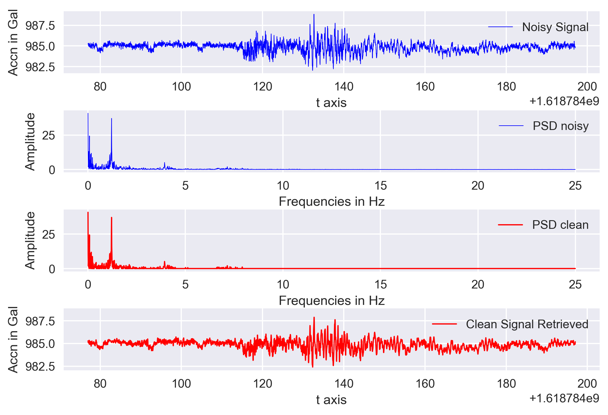
I have a recording of the accelerometer data using the PhidgetSpatial Precision 0/0/3 High Resolution. I converted that into Miniseed format for easy analysis.
# -*- coding: utf-8 -*-
# ======================================================================================================================================================
"""
Created on Thu Apr 29 12:41:26 2021

@author: Utpal Kumar (IES, Academia Sinica)
"""
# ======================================================================================================================================================

import numpy as np
import matplotlib.pyplot as plt
plt.rcParams['figure.figsize'] = [10,6]
plt.rcParams.update({'font.size': 18})
plt.style.use('seaborn')
from obspy import read
from obspy.core import UTCDateTime


otime = UTCDateTime('2021-04-18T22:14:37') #eq origin

filenameZ = 'TW-RCEC7A-BNZ.mseed'

stZ = read(filenameZ)
streams = [stZ.copy()]
traces = []
for st in streams:
    tr = st[0].trim(otime, otime+120)
    traces.append(tr)

delta = stZ[0].stats.delta
starttime = np.datetime64(stZ[0].stats.starttime)
endtime = np.datetime64(stZ[0].stats.endtime)
signalZ = traces[0].data/10**6
minsignal, maxsignal = signalZ.min(), signalZ.max()

t = traces[0].times("utcdatetime")

## Compute Fourier Transform
n = len(t)
fhat = np.fft.fft(signalZ, n) #computes the fft
psd = fhat * np.conj(fhat)/n
freq = (1/(delta*n)) * np.arange(n) #frequency array
idxs_half = np.arange(1, np.floor(n/2), dtype=np.int32) #first half index
psd_real = np.abs(psd[idxs_half]) #amplitude for first half


## Filter out noise
sort_psd = np.sort(psd_real)[::-1]
# print(len(sort_psd))
threshold = sort_psd[300]
psd_idxs = psd > threshold #array of 0 and 1
psd_clean = psd * psd_idxs #zero out all the unnecessary powers
fhat_clean = psd_idxs * fhat #used to retrieve the signal

signal_filtered = np.fft.ifft(fhat_clean) #inverse fourier transform


## Visualization
fig, ax = plt.subplots(4,1)
ax[0].plot(t, signalZ, color='b', lw=0.5, label='Noisy Signal')
ax[0].set_xlabel('t axis')
ax[0].set_ylabel('Accn in Gal')
ax[0].legend()

ax[1].plot(freq[idxs_half], np.abs(psd[idxs_half]), color='b', lw=0.5, label='PSD noisy')
ax[1].set_xlabel('Frequencies in Hz')
ax[1].set_ylabel('Amplitude')
ax[1].legend()

ax[2].plot(freq[idxs_half], np.abs(psd_clean[idxs_half]), color='r', lw=1, label='PSD clean')
ax[2].set_xlabel('Frequencies in Hz')
ax[2].set_ylabel('Amplitude')
ax[2].legend()

ax[3].plot(t, signal_filtered, color='r', lw=1, label='Clean Signal Retrieved')
ax[3].set_ylim([minsignal, maxsignal])
ax[3].set_xlabel('t axis')
ax[3].set_ylabel('Accn in Gal')
ax[3].legend()

plt.subplots_adjust(hspace=0.6)
plt.savefig('real-signal-analysis.png', bbox_inches='tight', dpi=300)
Obspy based filter
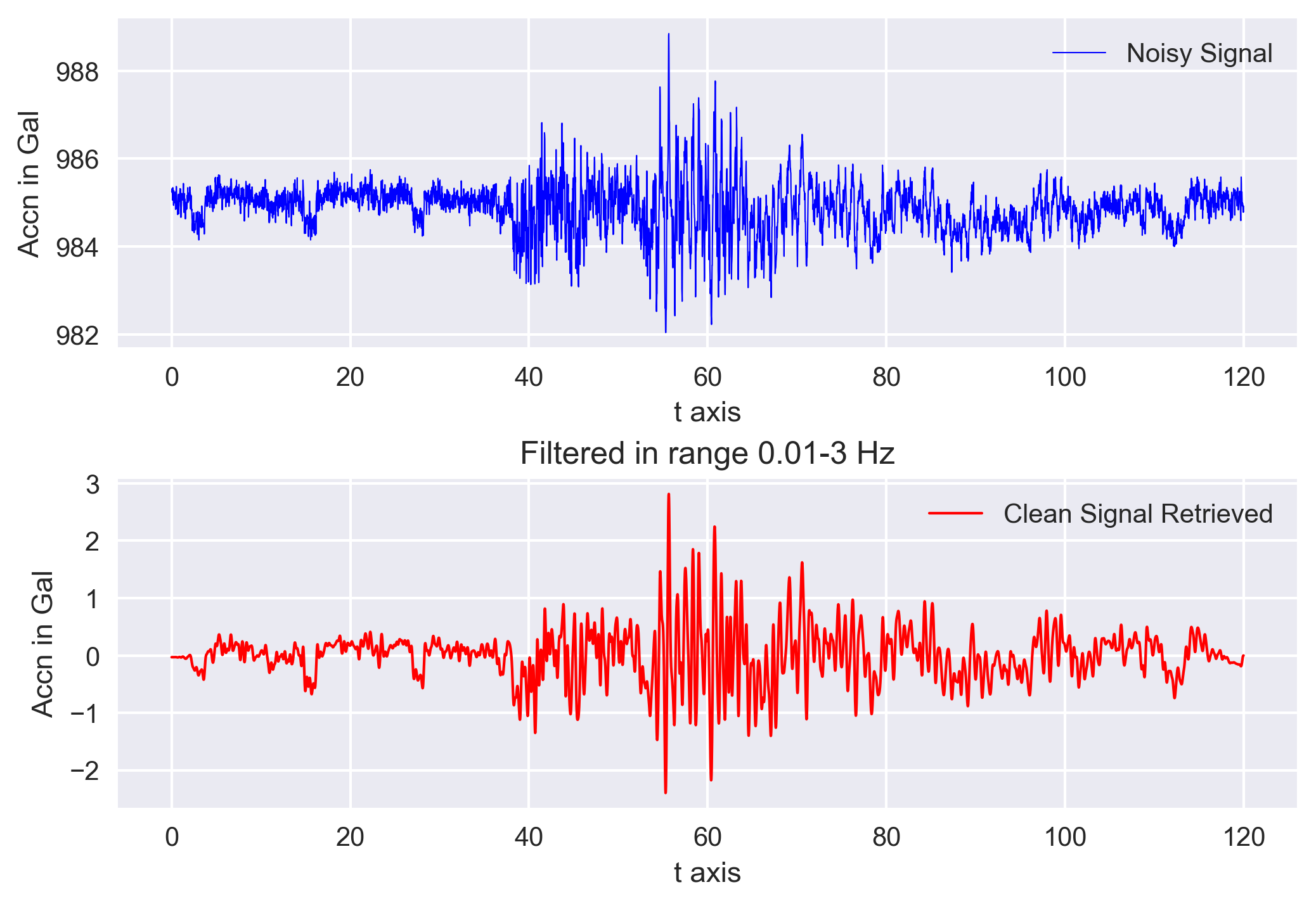
Obspy made our task much easier by introducing the filter functions. Here, I made use of the Butterworth-Bandpass filter. For details about different kinds of filters, you can see its documentation.
In this example, I used pass band low corner frequency of 0.01 and high corner frequency of 3 Hz based on the frequency spectrum obtained above.
import pandas as pd
import os, sys
import numpy as np
import matplotlib.pyplot as plt
plt.rcParams['figure.figsize'] = [10,6]
plt.rcParams.update({'font.size': 18})
plt.style.use('seaborn')
from obspy import read
from obspy.core import UTCDateTime

otime = UTCDateTime('2021-04-18T22:14:37') #eq origin

filenameZ = 'TW-RCEC7A-BNZ.mseed'

stZ = read(filenameZ)
streams = [stZ.copy()]
traces = []
for st in streams:
    tr = st[0].trim(otime, otime+120)
    traces.append(tr)


signalZ = traces[0].data/10**6
minsignal, maxsignal = signalZ.min(), signalZ.max()

t = np.arange(0, traces[0].stats.npts / traces[0].stats.sampling_rate, traces[0].stats.delta)

# Filtering with a lowpass on a copy of the original Trace
freqmin = 0.01
freqmax = 3
tr_filt = traces[0].copy()
tr_filt.detrend("linear")
tr_filt.taper(max_percentage=0.05, type='hann')
tr_filt.filter("bandpass", freqmin=freqmin,
                          freqmax=freqmax, corners=4, zerophase=True)
print(tr_filt.data/10**6)
signal_filtered = tr_filt.data/10**6

## Visualization
fig, ax = plt.subplots(2,1)
ax[0].plot(t, signalZ, color='b', lw=0.5, label='Noisy Signal')
ax[0].set_xlabel('t axis')
ax[0].set_ylabel('Accn in Gal')
ax[0].legend()


ax[1].plot(t, signal_filtered, color='r', lw=1, label='Clean Signal Retrieved')
ax[1].set_xlabel('t axis')
ax[1].set_ylabel('Accn in Gal')
ax[1].set_title(f"Filtered in range {freqmin}-{freqmax} Hz")
ax[1].legend()

plt.subplots_adjust(hspace=0.4)
plt.savefig('real-signal-analysis.png', bbox_inches='tight', dpi=300)
Conclusions
In this post, we only used the basic kind of filter to remove the noise. With the advanced filter, we can have more control in the removal of the frequencies but the overall concept is very similar. In the next post, we will see how we can use wavelets to remove the noise.
Recap
- Denoise in the frequency domain. FFT → threshold the power spectrum → inverse FFT keeps the strong frequency peaks and drops the broadband noise.
- It’s a mask, then a product.
psd > thresholdmakes a 0/1 mask; multiply it intofhatandifftback. - Two ways to set the threshold. A fixed power level (synthetic example) or “keep the top-N components” (
sort_psd[300]in the real-data example). - ObsPy filters are the practical route. A zero-phase Butterworth
bandpass(withdetrend+taperfirst) is the standard way to band-limit real seismic data. - Wavelets when frequencies overlap. FFT filtering assumes signal and noise separate in frequency; when they don’t, reach for wavelets.
Where to go next
- Next step — wavelet denoising: Signal denoising using MATLAB wavelet analysis
- Why wavelets beat Fourier for non-stationary signals: Towards multi-resolution analysis with the wavelet transform
numpy.fft.fftdocs: numpy.org/doc/stable/reference/generated/numpy.fft.fft.html- ObsPy
Stream.filterdocs: docs.obspy.org — Stream.filter
References
- Stein, S., & Wysession, M. (2009). An Introduction to Seismology, Earthquakes, and Earth Structure. Blackwell Publishing.
Disclaimer of liability
The information provided by the Earth Inversion is made available for educational purposes only.
Whilst we endeavor to keep the information up-to-date and correct. Earth Inversion makes no representations or warranties of any kind, express or implied about the completeness, accuracy, reliability, suitability or availability with respect to the website or the information, products, services or related graphics content on the website for any purpose.
UNDER NO CIRCUMSTANCE SHALL WE HAVE ANY LIABILITY TO YOU FOR ANY LOSS OR DAMAGE OF ANY KIND INCURRED AS A RESULT OF THE USE OF THE SITE OR RELIANCE ON ANY INFORMATION PROVIDED ON THE SITE. ANY RELIANCE YOU PLACED ON SUCH MATERIAL IS THEREFORE STRICTLY AT YOUR OWN RISK.
Leave a comment