How to implement the iterative Newton–Raphson method to find roots of a function in Python

We often opt for the iterative methods for solving a number of problems in geosciences.

The goal of such an iterative scheme is to achieve convergence (for root finding or solving a system of linear equations) or divergence (applications using differential equations). In computer programming, we usually use a “for loop” to implement an iteration procedure.

Some the iterative methods I have covered so far are Monte Carlo methods and Genetic algorithm in the context of the earthquake location problem.

What is the Newton–Raphson method?

The Newton–Raphson method (commonly known as Newton’s method) is developed for finding roots of a given function or polynomial iteratively.

Consider a non-linear equation, where we seek to find the root $x_r$

The Newton–Raphson method is an iterative scheme that relies on an initial guess, $x_0$, for the value of the root. From the initial guess, subsequent guesses are obtained iteratively until the scheme either converges to the root $x_r$ or the scheme diverges and we seek another initial guess. The sequence of guesses are obtained from the slope of the function.

This gives the Newton–Raphson iterative relation (Kutz, 2013):

Notice that in the above equation, the scheme fails if $f’(x_n) = 0$. In general, if the initial guess is sufficiently close to $x_r$, the scheme converges. See Burden and Faires (1997) for details on the conditions for convergence.

Python Example 1

Let us now implement Newton’s method for finding root of the problem:

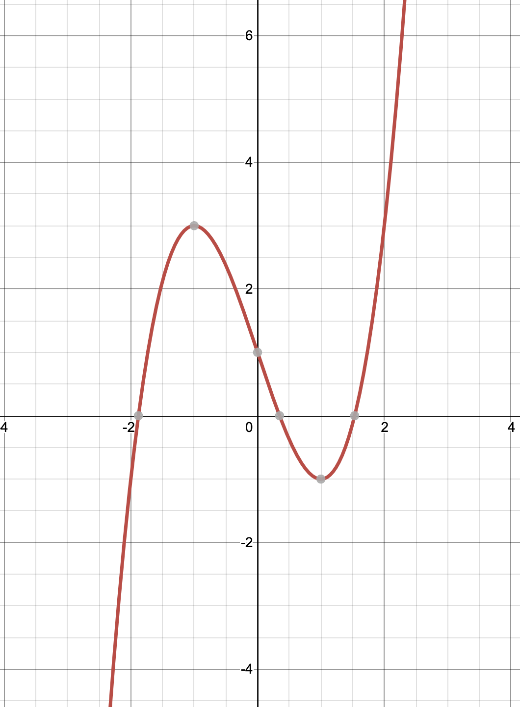
For this equation, we have $f(x) = x^3 - 3x + 1$ and $f’(x) = 3x^2 - 3$. Hence, the Newton’s formula becomes:

import numpy as np
import matplotlib.pyplot as plt
plt.style.use('seaborn')

x = np.zeros((1000, 1))

x[0] = 5.0  # initial guess

fig, ax = plt.subplots(1, 1)
for j in range(1000):
    # x_{n+1} = x_n - \frac{x^3 - 3x + 1}{3x^2 - 3}
    x[j+1] = x[j] - (x[j]**3 - 3*x[j] + 1)/(3*x[j]**2 - 3)

    # f(x) = x^3 - 3x + 1
    func = x[j+1]**3 - 3*x[j+1] + 1

    ax.plot(x[j], func, 'o', color='b')

    # termination criteria
    if np.abs(func) < 10**-6:
        break

plt.gca().invert_xaxis()
ax.set_xlabel('x')
ax.set_ylabel('f(x)')
plt.savefig('example1.png', dpi=300, bbox_inches='tight')
plt.close()
print(f"The root of the function is: {x[j+1]}")
print(f"Function value at the root: {func}")

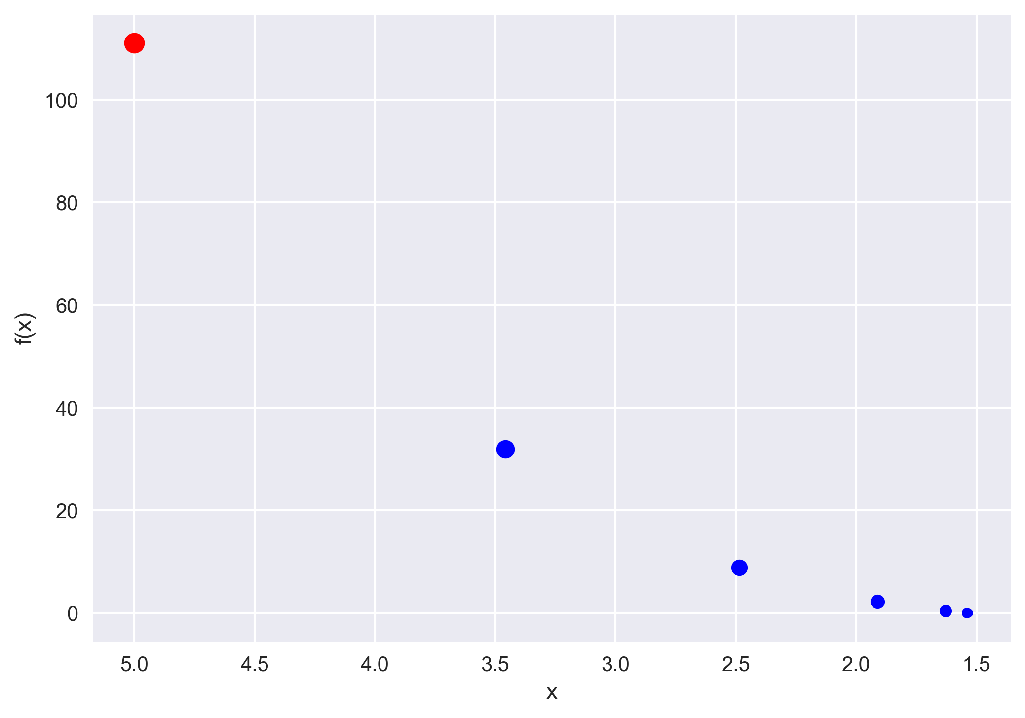
The root of the function is: [1.5320889]
Function value at the root: [4.00197986e-08]

Python Example 2

Let us now borrow a function used by Kutz, 2013.

The derivative of this function is $f’(x) = exp(x) - sec^2(x)$, which leads to the Newton’s formula:

import numpy as np
import matplotlib.pyplot as plt
plt.style.use('seaborn')

x = np.zeros((1000, 1))

x[0] = 10.0  # initial guess

fig, ax = plt.subplots(1, 1)
for j in range(1000):
    # x_{n+1} = x_n - \frac{exp(x_n) - tan(x_n)}{exp(x_n) - sec^2(x_n)}
    x[j+1] = x[j] - (np.exp(x[j]) - np.tan(x[j])) / \
        (np.exp(x[j]) - (1/np.cos(x[j]))**2)

    # f(x) = exp(x) - tan(x)
    func = (np.exp(x[j+1]) - np.tan(x[j+1]))

    ax.plot(x[j], func, 'o', color='b')

    # termination criteria
    if np.abs(func) < 10**-6:
        break

plt.gca().invert_xaxis()
ax.set_xlabel('x')
ax.set_ylabel('f(x)')
plt.savefig('example2.png', dpi=300, bbox_inches='tight')
plt.close()
print(f"The root of the function is: {x[j+1]}")
print(f"Function value at the root: {func}")

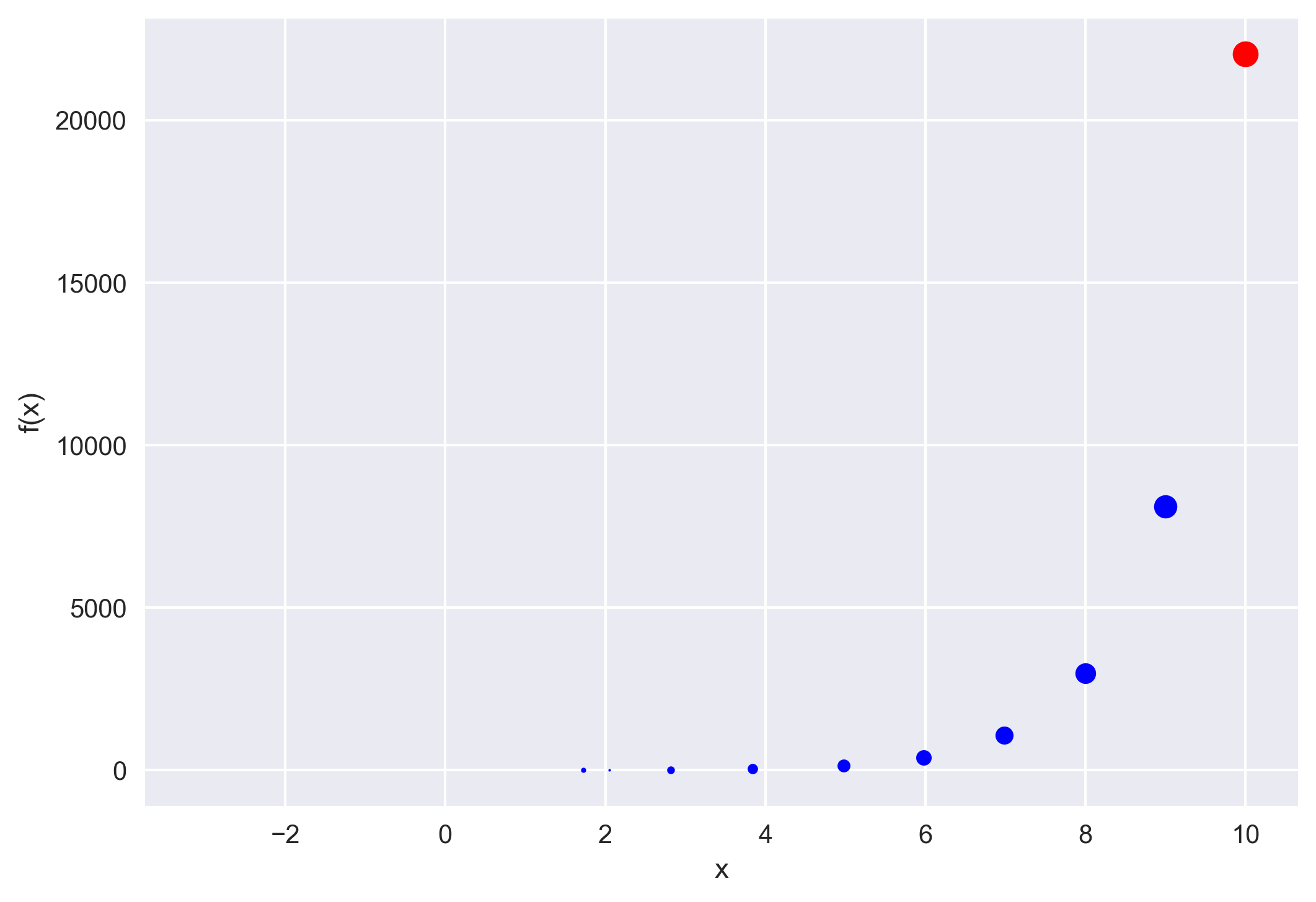
The root of the function is: [-3.0964123]
Function value at the root: [-7.14244983e-11]

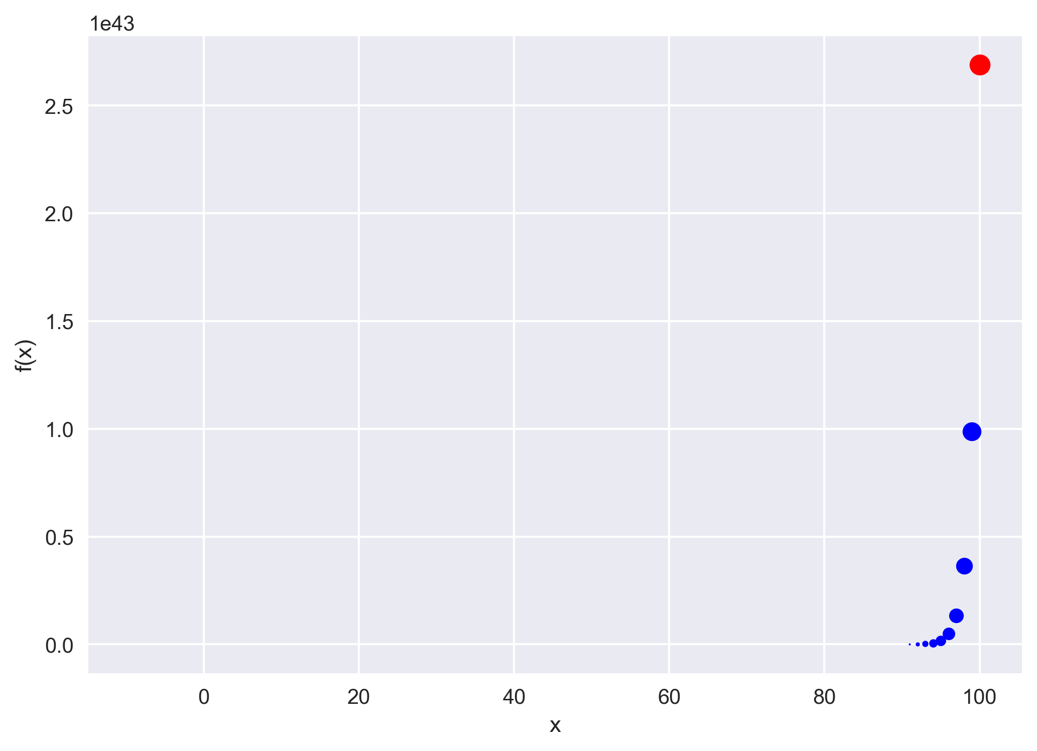
Now, let us run the above code for the initial guess of x[0] = 100.0.

Conclusions

The Newton’s method is very fast to converge to the solution for a sufficiently close guess. However, if we have a bad guess then it does not converge at all.

Recap

• One step, one tangent. $x_{n+1} = x_n - f(x_n)/f’(x_n)$ follows the tangent at the current guess down to the x-axis.
• Fast — when it works. Near the root, convergence is quadratic (the error roughly squares each step), so only a handful of iterations are needed.
• Two failure modes. It breaks when $f’(x_n) = 0$ (flat tangent, division by zero) and can diverge from a poor initial guess — exactly what the x[0] = 100.0 example shows.

• Stop on a small residual. The loop terminates when $

  f(x)

  $ drops below a tolerance ($10^{-6}$ here), meaning the guess is effectively a root.

Where to go next

• scipy.optimize.newton docs: docs.scipy.org/doc/scipy/reference/generated/scipy.optimize.newton.html
• Root-finding in action — the shooting method for BVPs: Solving boundary value problems using the shooting method
• Related iterative schemes: Euler method · Runge–Kutta method

References

1. Kutz, J. N. (2013). Data-driven modeling & scientific computation: methods for complex systems & big data. Oxford University Press.
2. R. L. Burden and J. D. Faires, Numerical Analysis (Brooks/Cole, 1997).