Towards multi-resolution analysis with wavelet transform
We will learn the basic concepts of wavelet tranform and multi-resolution analysis starting from the Fourier Transform, and Gabor Transform.
We have used Fourier transform in several past posts. It is one of the most important and foundational methods for the analysis of signals. It can capture all the frequency content of the signal with the transform, but the transform fails to capture the exact moment in time when various frequencies are actually present. In other words, it is taking some signal in either space or time and writing it into its frequency components.
It is an excellent tool for characterizing stationary or periodic signals. The stationary signals are simply the repeated measurements in time that is an average value that does not change in time. Most of our real-world signals do not satisfy this criterion.
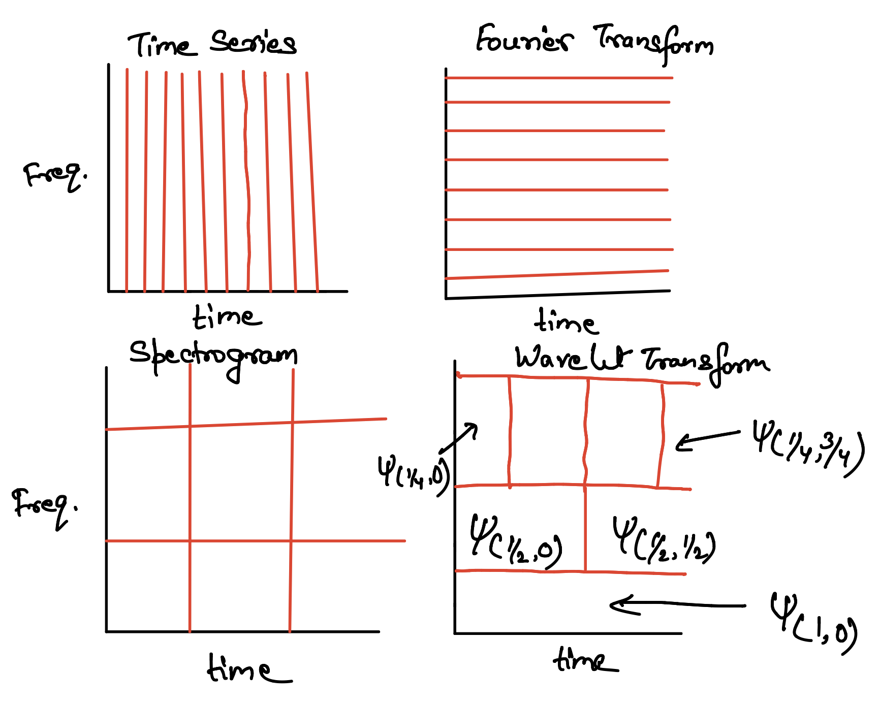
When we look at our signal in the time domain, we can precisely tell where we are in terms of time, but we have absolutely no idea about the frequency of that instant. When we look at our signals in the frequency domain, we have an absolute understanding of the frequency at a particular instant, but we have no idea about the time. For example, if you look at audio signals, we know in the frequency domain what frequencies were played, but we can’t tell what time it was planned.
Gabor transform allows us to prepare a spectrogram that essentially is the time-frequency plot. Fourier transform makes sense for the signal, which is entirely periodic, but most of that, your physical signals are not periodic, they do contain frequencies, but those frequencies are not regularly repeating at time.
Gabor transform and the spectrogram
The inability of the Fourier transform to localize the signal in both the time in the frequency domain has been realized very early in the development of radar and sonar detection technology. The Hungarian physicist Gabor Denes proposed a method that involves the simple modification of the Fourier transform. This is popularly known as the short-time Fourier transform. The Gabor method trades aways some measure of accuracy in both the time and frequency domain to simultaneously obtain both time and frequency resolution.
What Gabor transform do is to take Gaussian window and convolve that with the Fourier transform, sliding across the signal. Essentially we are computing the weighted Fourier transform only in the window and moving that window across the signal in time.
\begin{equation} G (f) = \hat{f}_g(t,\omega) \end{equation}
\begin{equation} = \int_{-\infty}^{\infty} f(\tau)e^{-i\omega \tau} g(t-\tau) d\tau \end{equation}
where \(g(\tau)\) is the Gaussian Gabor window. In the above equation, we can see that the Gabor transform is just a Fourier transform weighted by the Gaussian function. So it gives us some resolution of the frequencies and some resolution of the time.
Gabor method is limited by the time filtering. The time window filters out the time behavior of the signal in a window centered at Tao and width a. Any portion of the signal with a wavelength longer than the window size is completely lost. If we try to capture a longer period of wavelengths, we lose the signal’s time resolution. Here, the fixed window size imposes a limitation on the level of time-frequency resolution that can be obtained.
Wavelet Transform and Multi-resolution analysis
A simple modification to the Gabor method is to allow the window scaling to vary. We can first target the low-frequency components and then keep broadening the window size. This approach, which is the wavelet analysis approach, can give us excellent time and frequency resolution of the signal. Another advantage of the website analysis approach is that, unlike Fourier analysis, there are a wide variety of mother wavelets that can be constructed. The mother wavelet is generally designed based on the given problem.
Unlike the Fourier transform, which represents the signal as a series of sines and cosines, the wavelet is simply another expansion basis for representing a given signal.
The principle for wavelet transform is quite simple. We first split the signal into a bunch of smaller signals by translating the wavelet over the entire time domain of the signal. Then the same signal is processed in different frequency bands by scaling the wavelet window. This approach is also called a multi-resolution analysis because we analyze the signal at multiple resolutions. A multi-resolution analysis is a method that gives a formal approach to constructing the signal with different resolution levels. It is a hierarchical grading of time and frequency information.
Please note that because of the uncertainty principle, we always have to give back either time or frequency information to gain the other information. Wavelet transform is tailored to obtain as much information in the region as necessary. For example, lower frequencies don’t need as much temporal information as high frequencies (it depends on your target), so we trade temporal information for the lower frequencies to obtain the frequency information.
The wavelet-based decomposition works similarly as the Fourier decomposition. In the Fourier decomposition, we would take a signal and project it on orthogonal basis (sines and cosines). But in wavelet-based decomposition, the orthogonal basis is not just going to be sines or cosines, but it will be a hierarchy of orthogonal functions that will become smaller and smaller in time or space.
We always start with the mother wavelet (say \(\psi (t)\)), which is just a shape to start with.
\begin{equation} \psi_{a,b}(t) = \frac{1}{\sqrt{a}}\psi (\frac{t-b}{a}) \end{equation}
If the function, \(\psi (t)\), is Gaussian, then b will be the translation parameter (slide the Gaussian from left to right), and \(a\) will be the scaling parameter that will make the wavelet bigger or smaller (bigger a will make the wavelet smaller). So the increase in \(a\) will take us higher and higher in levels, and the increase in \(b\) will slide us across the time.
We can write the wavelet transform as \begin{equation} W_{\psi}(f)(a,b) = < f(t), \psi_{a,b}(t) > \end{equation}
The oldest wavelet (1910) designed is the Haar wavelet (\(\psi_{1,0}\)):

The \(\psi_{1,0}\) is the mother wavelet and we can obtain all sorts of variations from it - \(\psi_{1/2,1/2}\), \(\psi_{1/2,0}\), etc. All these wavelets are orthogonal in nature. We can imagine that the bigger scaled wavelets such as \(\psi_{1,0}\), etc will extract the bigger features in the signal and the smaller wavelets such as \(\psi_{1/2,1/2}\), \(\psi_{1/2,0}\) will pull out smaller features.
Conclusions
We have started with the concept of Fourier transform, seen the basics of Gabor transform, and then finally delved slightly into the multi-resolution analysis with wavelets. In future posts, I will discuss the applications of wavelet analysis such as wavelet denoising, image compression, image denoising, etc.
References
- Kutz, J. N. (2013). Data-driven modeling & scientific computation: methods for complex systems & big data. Oxford University Press.
Disclaimer of liability
The information provided by the Earth Inversion is made available for educational purposes only.
Whilst we endeavor to keep the information up-to-date and correct. Earth Inversion makes no representations or warranties of any kind, express or implied about the completeness, accuracy, reliability, suitability or availability with respect to the website or the information, products, services or related graphics content on the website for any purpose.
UNDER NO CIRCUMSTANCE SHALL WE HAVE ANY LIABILITY TO YOU FOR ANY LOSS OR DAMAGE OF ANY KIND INCURRED AS A RESULT OF THE USE OF THE SITE OR RELIANCE ON ANY INFORMATION PROVIDED ON THE SITE. ANY RELIANCE YOU PLACED ON SUCH MATERIAL IS THEREFORE STRICTLY AT YOUR OWN RISK.