Hypothesis test for the significance of linear trend using the Monte Carlo simulations (codes included)

Introduction

Monte Carlo (named based on a town famous for gambling) is a method for estimating the value of unknown quantity based on the principles of inferential statistics. Inferential statistics can be explained based on the concepts of two keywords – population and sample. Population is simply the collection of all the possibilities for any quantity (an infinitely large set) and the sample is the proper subset of the population such as the data we collect for any event. We make the inference about the population based on the samples we have. It is important for the samples to be random otherwise it might not be good enough to represent the population.

Monte Carlo Simulations is widely used in optimization, numerical integration, and risk-based decision making. Here, we will learn how to use it to test the hypothesis for the significance of the trend. I have covered Monte Carlo simulations to test if the correlation value of 0.4 is significant for sample size of 10 in our previous post.

Data

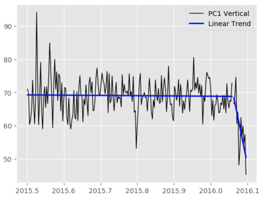
We have two data with two seemingly different trend. Here we want to statistically estimate if the trend of second data is significantly different.

Hypothesis Testing

We pose a null hypothesis and enquire that given that the null hypothesis is true, how likely is the observed pattern of results? This likelihood is known as the p-value, and indicates the statistical significance of the observed pattern of results. If the p-value is less than some predetermined threshold (say 0.05), we reject the null hypothesis. We can interpret the result of a statistical hypothesis test using a p-value. The p-value is the probability of observing the data, given the null hypothesis is true. A large probability means that the H0 or default assumption is likely. A small value, such as below 5% (0.05) suggests that it is not likely and that we can reject H0 in favor of H1.

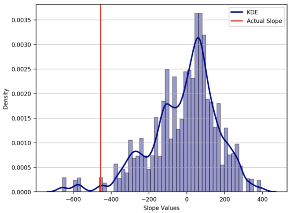
Here, let’s pose the null hypothesis that the second dataset come from the first distribution of data. So, the two dataset is interchangeable, so we can aggregate the two dataset and randomly sample data of the size of our second dataset and calculate the slope. The sample we select should be sequential, we only randomly select the starting point of the sample. We draw samples many times (10,000 in this case) to obtain a reliable probability distribution. We can then compare the resulting distribution with the actual slope value. We also calculate the p-value by counting the number of randomly sampled slope values that are more extreme than the actual observed value for the second data set and divide this by the total number of simulations ran. Here, we will utilize the modern computer to calculate the p-value instead of obtaining it analytically.

Monte Carlo Simulations

import matplotlib.pyplot as plt
import numpy as np
import scipy.io as sio
import matplotlib
import dec2dt
from toYearFraction import toYearFraction as tyf
from scipy import stats
import seaborn as sns

font = {'size'   : 8}
matplotlib.rc('font', **font)

st1=0
ed1=217

st2=205
ed2=217
len2=(ed2-st2)+1
matfiles=['pc1_U.mat']
mat=matfiles[0]
pcdata=sio.loadmat(mat)
pc_tdata=np.transpose(np.array(pcdata['tdata']))
pc=np.array(pcdata['pcdata'])
pctime=[]
for i in range(len(pc_tdata)):
    pctime.append(dec2dt.dec2dt(pc_tdata[i]))
pctime=np.array(pctime)
comp=mat.split('.')[0].split("_")[1]
mode=mat[2]
x1=np.array([pct[0] for pct in pc_tdata[st1:ed1]])
y1=np.array([p[0] for p in pc[st1:ed1]])

x2=np.array([pct[0] for pct in pc_tdata[st2:ed2]])
y2=np.array([p[0] for p in pc[st2:ed2]])
slope_actual, intercept_actual, r_value_actual, p_value_actual, std_err_actual = stats.linregress(x2,y2)
print(slope_actual,r_value_actual)
slopes=[]
for i in range(10000):
    rand_idx = np.random.randint(ed1-len2,size=1)[0]
    x1_rand=x1[rand_idx:rand_idx+len2]
    y1_rand=y1[rand_idx:rand_idx+len2]

    slope, intercept, r_value, p_value, std_err = stats.linregress(x1_rand,y1_rand)
    slopes.append(slope)
slopes=np.array(slopes)
pval = np.sum(np.abs(slopes) > np.abs(slope_actual))/ len(slopes)
plt.figure()
sns.distplot(slopes, hist=True, kde=True, bins='auto', color = 'darkblue', hist_kws={'edgecolor':'black'},kde_kws={'linewidth': 2, "label": "KDE"})
plt.grid(axis='y', alpha=0.75)
plt.axvline(x=slope_actual,c='r',label='Actual Slope')
plt.legend()
plt.ylabel('Density')
plt.xlabel('Slope Values')
plt.savefig('hypothesis_test_eof1.png'.format(mode,comp),dpi=200,bbox_inches='tight')

sns.distplot is on its way out. Seaborn deprecated distplot in v0.11 and it is scheduled for removal in v0.14.0 (it still runs with a warning in the current 0.13.x). Swap it for the modern axes-level replacement — sns.histplot(slopes, kde=True, color="darkblue", edgecolor="black") — or the figure-level sns.displot(...). The scipy.stats.linregress and numpy calls above are unchanged; linregress still unpacks to the same five values.

We have used the absolute value for the calculation of “pval” or p-value so that both positive and negative correlations count as “extreme”. This is referred to as a two-tailed test. Under the null hypothesis, we would expect to find slope values of that size or larger about 2% of the time. Thus, we have sufficient evidence to reject the null hypothesis. In other words, the actual slope value observed is deemed significantly different.

Recap

• A p-value answers: if the null hypothesis were true, how often would chance alone produce a result at least this extreme?
• Monte Carlo estimates it without any formula: build a null distribution by drawing many random no-trend samples, fit a slope to each, and compare.
• The p-value is the fraction of surrogate slopes as extreme as the observed one; using abs() makes it a two-tailed test (both large positive and large negative slopes count).
• Here about 2% of surrogates were that extreme, so with a 0.05 threshold the observed trend is significant — reject the null.
• The method is assumption-light (no need for normality or a known sampling distribution), which is why it is so widely used for messy real-world data.

Where to go next

• Understanding the Metropolis–Hastings algorithm — Monte Carlo that samples a distribution rather than testing a hypothesis.
• Monte Carlo methods and the earthquake location problem — the same random-sampling idea used for inversion.
• Time-series analysis: filtering and smoothing data — prepare a series before testing it for trends.