How to analyze a huge data file with Pandas (codes included)

import pandas as pd
import os, sys, glob
import numpy as np
import enum # Enum for size units
import time
import matplotlib.pyplot as plt
from datetime import datetime as dt


class SIZE_UNIT(enum.Enum):
   BYTES = 1
   KB = 2
   MB = 3
   GB = 4
def convert_unit(size_in_bytes, unit):
   """ Convert the size from bytes to other units like KB, MB or GB"""
   if unit == SIZE_UNIT.KB:
       return size_in_bytes/1024
   elif unit == SIZE_UNIT.MB:
       return size_in_bytes/(1024*1024)
   elif unit == SIZE_UNIT.GB:
       return size_in_bytes/(1024*1024*1024)
   else:
       return size_in_bytes


def get_file_size(file_name, size_type = SIZE_UNIT.BYTES ):
   """ Get file in size in given unit like KB, MB or GB"""
   size = os.path.getsize(file_name)
   return convert_unit(size, size_type)

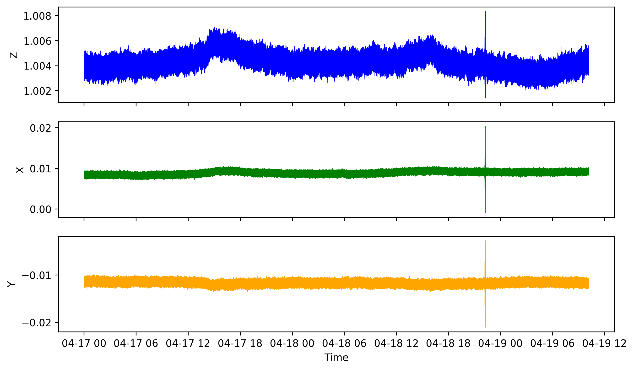
## Plot the data
def plot_data(datetime_array, z_array, x_array, y_array, output="data_plot_ts.png"):
    # Create figure and plot space
    fig, ax = plt.subplots(3, 1, figsize=(10, 6), sharex=True)
    
    # Add x-axis and y-axis
    ax[0].plot(datetime_array,
                z_array,
                color='blue', lw=0.5)
    ax[0].set_ylabel("Z")
    
    ax[1].plot(datetime_array,
                x_array,
                color='green', lw=0.5)
    ax[1].set_ylabel("X")
    
    ax[2].plot(datetime_array,
                y_array,
                color='orange', lw=0.5)
    ax[2].set_ylabel("Y")
    
    plt.xlabel("Time")
    plt.savefig(output, bbox_inches='tight', dpi=300)
    plt.close('all')
    

datalocation = "data"
all_data = glob.glob(os.path.join(datalocation, "*.csv"))
# print(all_data)

filename = all_data[0]
# print(filename)


filesize = get_file_size(filename, SIZE_UNIT.MB)
print(f"{filename} is of size {filesize:.2f} MB")


use_plain_python = 1
if use_plain_python: 
    chunksize = 10**6
    print("Buffer size is: ", convert_unit(chunksize, SIZE_UNIT.MB)) #depends on your RAM size
    starttime = time.perf_counter()
    x_array = np.array([],dtype=np.float64)
    y_array = np.array([],dtype=np.float64)
    z_array = np.array([],dtype=np.float64)
    datetime_array = np.array([],dtype='datetime64')
    with open(filename, mode= 'r', buffering=chunksize) as f:
        for fchunk in f:
            print(fchunk, end='')
            dtime, xx, yy, zz = fchunk.split(",")
            date_time_obj = dt.strptime(dtime, '%Y-%m-%d %H:%M:%S.%f')
            datetime_array = np.append(datetime_array, date_time_obj)
            x_array = np.append(x_array, np.array(xx))
            y_array = np.append(y_array, np.array(yy))
            z_array = np.append(z_array, np.array(zz))
       
            
    
    print(f"---Finished in {time.perf_counter()-starttime:.2f} secs---")
    plot_data(datetime_array, z_array, x_array, y_array, output="data_plot_ts_plain_python.png")

use_pandas = 1
if use_pandas:
    chunksize = 10 ** 6
    starttime = time.perf_counter()
    x_array = np.array([],dtype=np.float64)
    y_array = np.array([],dtype=np.float64)
    z_array = np.array([],dtype=np.float64)
    datetime_array = np.array([],dtype='datetime64')
    for df in pd.read_csv(filename, chunksize=chunksize, names=[
                         'Datetime', "X", "Y", "Z"], dtype={"Datetime": "str", "X": np.float64,"Y": np.float64,"Z": np.float64}):
        print(df.head(1))
        df["Datetime"] = pd.to_datetime(df["Datetime"])
        datetime_array = np.append(datetime_array, df["Datetime"].values)
        x_array = np.append(x_array, df['X'].values)
        y_array = np.append(y_array, df['Y'].values)
        z_array = np.append(z_array, df['Z'].values)
    print(datetime_array.shape, x_array.shape, y_array.shape, z_array.shape)
    print(f"---Finished in {time.perf_counter()-starttime:.2f} secs---")
    plot_data(datetime_array, z_array, x_array, y_array, output="data_plot_ts_pandas.png")