Maximum likelihood estimation for the regression parameters
The maximum likelihood method is popular for obtaining the value of parameters that makes the probability of obtaining the data given a model maximum. In other words, the goal of this method is to find an optimal way to fit a model to the data.
Key idea — pick the parameters that make your data most probable. Maximum likelihood estimation flips the usual question around: instead of asking “given these parameters, how likely is the data?”, it asks “which parameters make the data I actually observed most likely?” Two practical moves make it work: we maximize the log-likelihood (a product of many tiny probabilities becomes a numerically-stable sum), and because optimizers minimize, we minimize the negative log-likelihood. The punchline of this post: when the errors are Gaussian, MLE gives you exactly the least-squares answer.
Introduction
Let us assume that the parameter we want to estimate is $\theta$. Then we collect some data $x_1, x_2, …, x_n$ as random samples (it needs to be independent and identically distributed) from probability density function (pdf). So, what is the most likely value of $\theta$, given the data we have observed?
Let us define a likelihood function: \(\begin{aligned} L (\theta | x_1, x_2, ..., x_n) = f(x_1, x_2, ..., x_n | \theta) \end{aligned}\)
\[\begin{aligned} = f(x_1| \theta) ... f(x_n | \theta) \end{aligned}\] \[\begin{aligned} = \prod_{i=1}^n f(x_i|\theta) \end{aligned}\]We can write the Likelihood function as a product of pdf’s of x given that x’s are independent. The value of $\theta$ that maximimizes the likelihood function is called Maximum Likelihood Estimator.
You will see that in the later examples that we will numerically maximize the log (natural log) of the maximum likelihood function rather than the MLE itself. This is because MLE is a product of probabilities of N data samples and can become very small for large N and hence computationally infeasible. Taking the log of the product converts it into the sum of many terms. Also, the log function is monotonic, thus can be applied on the MLE function without changing its behaviour (increasing or decreasing).
\[\begin{aligned} log(a.b) = log(a) + log(b) \end{aligned}\]The illustration of the estimation procedure
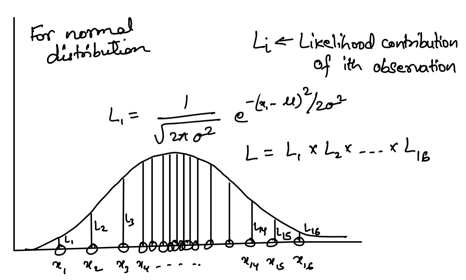
Let us assume that the data comes from the Normal distribution. We know the pdf of the normal distribution.
\[\begin{aligned} f(x) = \frac{1}{\sqrt{2\pi \sigma^2}}e^{-(x-\mu)^2/2\sigma^2} \end{aligned}\]The likelihood function becomes:
\[\begin{aligned} L = \prod_{i=1}^N f(x) \end{aligned}\]Then the problem is to find the MLE of mean ($\mu$), and standard deviation ($\sigma$) that maximizes the likelihood function.
We find the maximum by setting the derivatives equal to zero:
\[\begin{aligned} \frac{d\ln(L)}{d\mu} &= 0 \\ \frac{d\ln(L)}{d\sigma} &= 0 \end{aligned}\]Least-squares vs the Maximum Likelihood Estimation
Let us consider a linear regression problem. The expected value of the function, y is
\[\begin{aligned} E[Y_i] = \beta_0 + \beta_1 x_i \end{aligned}\]The residuals from the observation are: \(\begin{aligned} r_i = y_i - E[Y_i] \end{aligned}\)
In the method of the least-squares, we find the values for the parameters that makes the sum of the squared residuals as small as possible. The assumption here is that the residuals are obtained from the normal distribution (or the error terms are normal). In contrast, the maximum likelihood method can be applied to models from any probability distribution.
Why they coincide for Gaussian errors. If the residuals are normal, each term of the log-likelihood is $-\tfrac{(y_i - \hat y_i)^2}{2\sigma^2}$ plus a constant. Summing over the data, maximizing that log-likelihood is the same as minimizing $\sum (y_i - \hat y_i)^2$ — the least-squares objective. So least squares is just MLE under a normal-error assumption; MLE is the more general tool because you can swap in any distribution.
Estimation of regression paramters
\(\begin{aligned} y = \beta_0 + \beta_1 x + u \end{aligned}\) where, $u$ is the error term. Let us make an assumption that $u$ follows the normal distribution with mean 0 and variance $\sigma^2$.
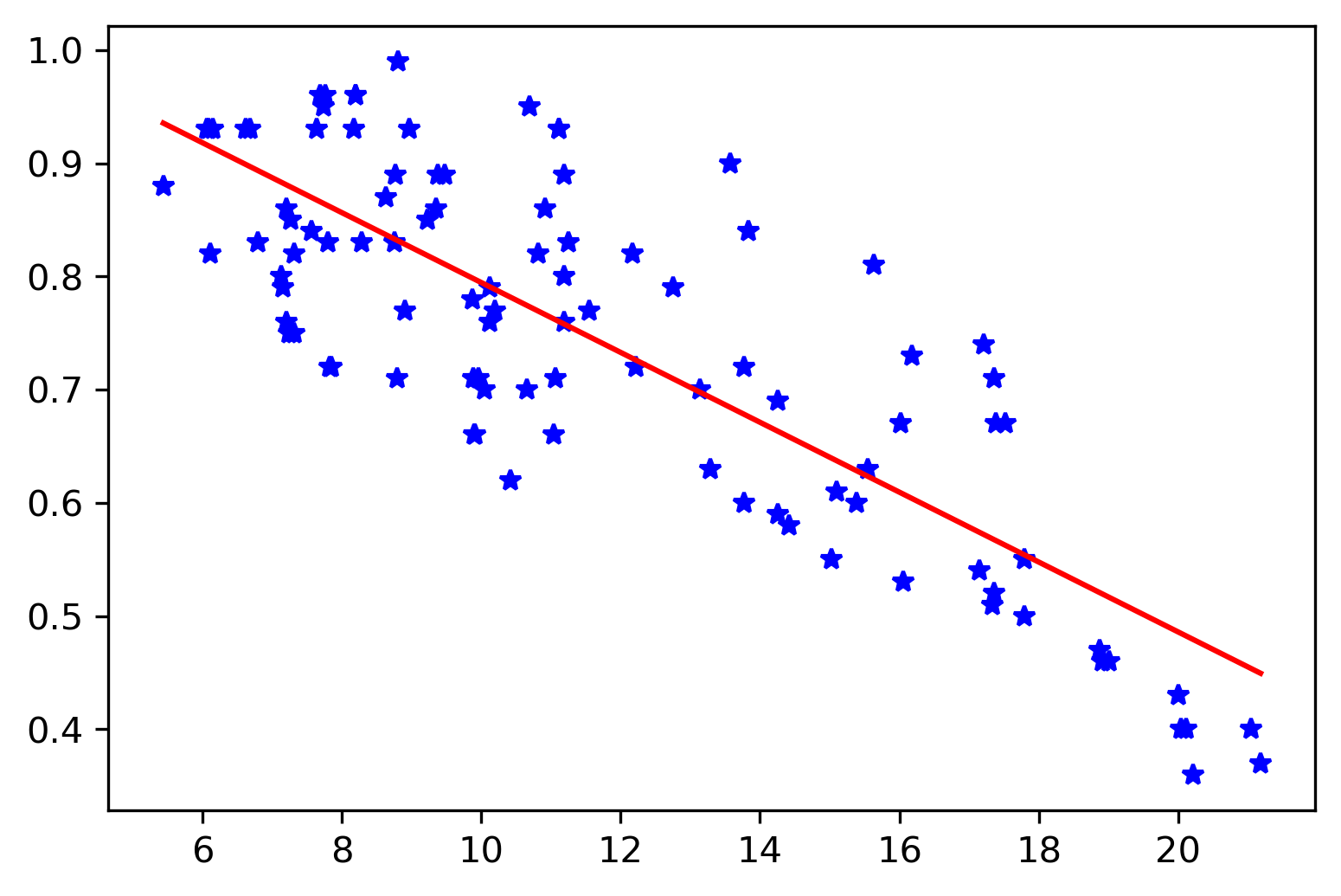
I obtained the dataset from Kaggle for a relationship between humidity and temperature. Download from here. This is simply for demonstration purpose. You can apply it on any dataset.
Import libraries and dataset
import numpy as np
from scipy.optimize import minimize
import scipy.stats as stats
import pandas as pd
import statsmodels. api as sm
import matplotlib.pyplot as plt

df = pd.read_csv('weatherHistory.csv')
x = df['Temperature (C)'][:100]
y = df['Humidity'][:100]

fig, ax = plt.subplots()
ax.plot(x,y, 'b*')
plt.savefig('temp_humidity.png',bbox_inches='tight', dpi=300)
plt.close()

Apply the least-squares method to obtain the relationship
We first define the least-squares model for the regression problem, and then attempt to fit it with our data.
x2 = sm.add_constant(x)
modl = sm.OLS(y,x2)
mod12=modl.fit()
print(mod12.summary())
                            OLS Regression Results
==============================================================================
Dep. Variable:               Humidity   R-squared:                       0.676
Model:                            OLS   Adj. R-squared:                  0.672
Method:                 Least Squares   F-statistic:                     204.1
Date:                Sun, 15 Aug 2021   Prob (F-statistic):           1.08e-25
Time:                        23:25:07   Log-Likelihood:                 98.943
No. Observations:                 100   AIC:                            -193.9
Df Residuals:                      98   BIC:                            -188.7
Df Model:                           1
Covariance Type:            nonrobust
===================================================================================
                      coef    std err          t      P>|t|      [0.025      0.975]
-----------------------------------------------------------------------------------
const               1.1034      0.027     41.118      0.000       1.050       1.157
Temperature (C)    -0.0309      0.002    -14.286      0.000      -0.035      -0.027
==============================================================================
Omnibus:                        6.966   Durbin-Watson:                   0.304
Prob(Omnibus):                  0.031   Jarque-Bera (JB):                4.780
Skew:                           0.391   Prob(JB):                       0.0916
Kurtosis:                       2.268   Cond. No.                         36.9
==============================================================================
We have obtained the best fit of the regression line with our dataset. We can obtain the error terms as:
## Error
e=mod12.resid
estd = np.std(e)

fig, ax = plt.subplots()
ax.plot(x,y, 'b*')

# plot the regression output
fig, ax = plt.subplots()
ax.plot(x,y, 'b*')
xx = np.linspace(np.min(x), np.max(x), 100)
yy =  mod12.params[1]* xx +  mod12.params.const
ax.plot(xx,yy, 'r-')
Here, we have obtained the regression relation from the least-squares method as: \(\begin{aligned} y = 1.1034 - 0.0309 x \end{aligned}\)
Now, let us try to obtain the same solution from the MLE method.
Apply the Maximum Likelihood Estimation method to obtain the relationship
We first define the likelihood function, lik. We assume that the error terms follow the Normal distribution and then we maximize the sum of the logs of the individual terms. Here, we use the minimize function from scipy. Hence, to obtain the maximum of L, we find the minimum of -L (remember that the log is a monotonic function or always increasing).
Further, we apply the contraints to keep the sigma to be positive for our convergence routine.
def lik(parameters, x, y):
    m = parameters[0]
    b = parameters[1]
    sigma = parameters[2]

    y_exp = m * x + b

    L = np.sum(np.log(norm.pdf(y - y_exp, loc = 0, scale=sigma)))
    return -L


def constraints(parameters):
    sigma = parameters[2]
    return sigma

cons = {
    'type': 'ineq',
    'fun': constraints
}
Add the norm import before running this. The lik function calls norm.pdf, but the imports above only bring in scipy.stats as stats. Add from scipy.stats import norm (or write stats.norm.pdf(...)) — otherwise you’ll hit NameError: name 'norm' is not defined.
Reading lik against the diagram: norm.pdf(y - y_exp, ...) is $f(x_i|\theta)$, np.log(...) turns the product into a sum, np.sum(...) adds the terms, and return -L is the negative so minimize can do the work.
We start with initial guess of the parameters: [2, 2, 2] (m, b, sigma). It doesn’t have to be accurate but simply reasonable.
lik_model = minimize(lik, np.array([2, 2, 2]), args=(x,y,), constraints=cons)
We have obtained a successful convergence of our optimization function.
     fun: -98.9428558904145
     jac: array([-0.0995636 , -0.00924873,  0.0002718 ])
 message: 'Optimization terminated successfully.'
    nfev: 387
     nit: 65
    njev: 65
  status: 0
 success: True
       x: array([-0.03087142,  1.10342661,  0.08996208])
The final parameters we obtained are: [-0.03087142, 1.10342661, 0.08996208]. This is almost the same as the ones we have obtained using the least-squares method (see above).
Quick check: Why does lik return -L instead of L?
fig, ax = plt.subplots()
ax.plot(x,y, 'b*')
xx = np.linspace(np.min(x), np.max(x), 100)
yy = lik_model.x[0] * xx +  lik_model.x[1]
ax.plot(xx,yy, 'r-')
plt.savefig('temp_humidity_regression.png',bbox_inches='tight', dpi=300)
plt.close()
Conclusions
In this post, we have learnt the basics of Maximum Likelihood Estimation method. We then solved a regression problem using MLE and compared it with the least-squares method. Using a similar approach, we can estimate parameters for several models (including non-linear ones) using MLE.
Recap
- MLE = most-probable parameters. Choose the parameter values that maximize the likelihood of the observed data.
- Work in log space. The likelihood is a product of pdfs; take the log to turn it into a stable sum and dodge numerical underflow.
- Minimize the negative. Since optimizers minimize, feed them $-\log L$ — that’s why the
likfunction returns-L. - Least squares is a special case. With Gaussian errors, maximizing the log-likelihood is minimizing the squared residuals — which is why the MLE fit (
y = 1.1034 - 0.0309 x) matches the OLS fit almost exactly. - MLE generalizes. Swap the normal pdf for any distribution and the same recipe estimates parameters for models least squares can’t handle.
Where to go next
scipy.optimize.minimizedocs: docs.scipy.org/doc/scipy/reference/generated/scipy.optimize.minimize.htmlscipy.stats.norm(the pdf used here): docs.scipy.org/doc/scipy/reference/generated/scipy.stats.norm.html- statsmodels OLS: statsmodels.org/stable/generated/statsmodels.regression.linear_model.OLS.html
References
- Maximum Likelihood Estimation-II (video): youtube.com/watch?v=5XITCyYmDug
Disclaimer of liability
The information provided by the Earth Inversion is made available for educational purposes only.
Whilst we endeavor to keep the information up-to-date and correct. Earth Inversion makes no representations or warranties of any kind, express or implied about the completeness, accuracy, reliability, suitability or availability with respect to the website or the information, products, services or related graphics content on the website for any purpose.
UNDER NO CIRCUMSTANCE SHALL WE HAVE ANY LIABILITY TO YOU FOR ANY LOSS OR DAMAGE OF ANY KIND INCURRED AS A RESULT OF THE USE OF THE SITE OR RELIANCE ON ANY INFORMATION PROVIDED ON THE SITE. ANY RELIANCE YOU PLACED ON SUCH MATERIAL IS THEREFORE STRICTLY AT YOUR OWN RISK.
Leave a comment