Solving boundary value problems using the shooting method
We have done several posts on the numerical problems such as using Euler method or Runge-Kutta methods for which the initial conditions are known. However, many physical applications do not have specified initial conditions, but rather some given boundary (constraint) conditions. The boundary value problems require information at the present time $(t = a)$ and a future time $(t = b)$. However, the time-stepping schemes developed previously in the case of initial value problems only require information about the starting time $t = a$. In this post, we will see a quick and easy way to solve these boundary value problems.
Key idea — turn a boundary value problem into a guessing game you can solve. A BVP fixes the value at both ends ($y(a)$ and $y(b)$), but our ODE solvers only march forward from one end. The shooting method bridges the gap: guess the missing initial slope, integrate forward as an ordinary initial value problem, and see how badly the endpoint misses the target $y(b)=\beta$. That miss is a function of your guess, so finding the right slope is just a root-finding problem — which we already know how to solve.
The Shooting Method
Let us begin by considering the generic boundary value problem:
\[\frac{d^2\vec{y}}{dt^2} = f(t,\vec{y},\frac{d\vec{y}}{dt})\]on $t \in [a, b]$ with the boundary conditions
\[y(a) = \alpha\] \[y(b) = \beta\]The stepping schemes considered thus far for second-order differential equations involve a choice of the initial conditions $y(a)$ and $y’(a)$. If we want to solve the above problem in a initial value problem approach, we can rewrite the above differential equation as below.
\[\frac{dy}{dt} = z\]For this equation, we need $y(a) = \alpha$, which is known.
\[\frac{dz}{dt} = f(t,\vec{y},\frac{d\vec{y}}{dt})\]For this equation, we need $z(a) = \kappa$, where $\kappa$ is unknown. Our goal here is to determine the value of $\kappa$ with the constrain $y(b) = \beta$.
For this, we can define a function $F = F(\kappa)$:
\[F(\kappa) = y(b) - \beta\]We have to find $\kappa$ such that $F(\kappa)=0$. This becomes a root finding problem and we know how to solve these problems (see Newton–Raphson method).
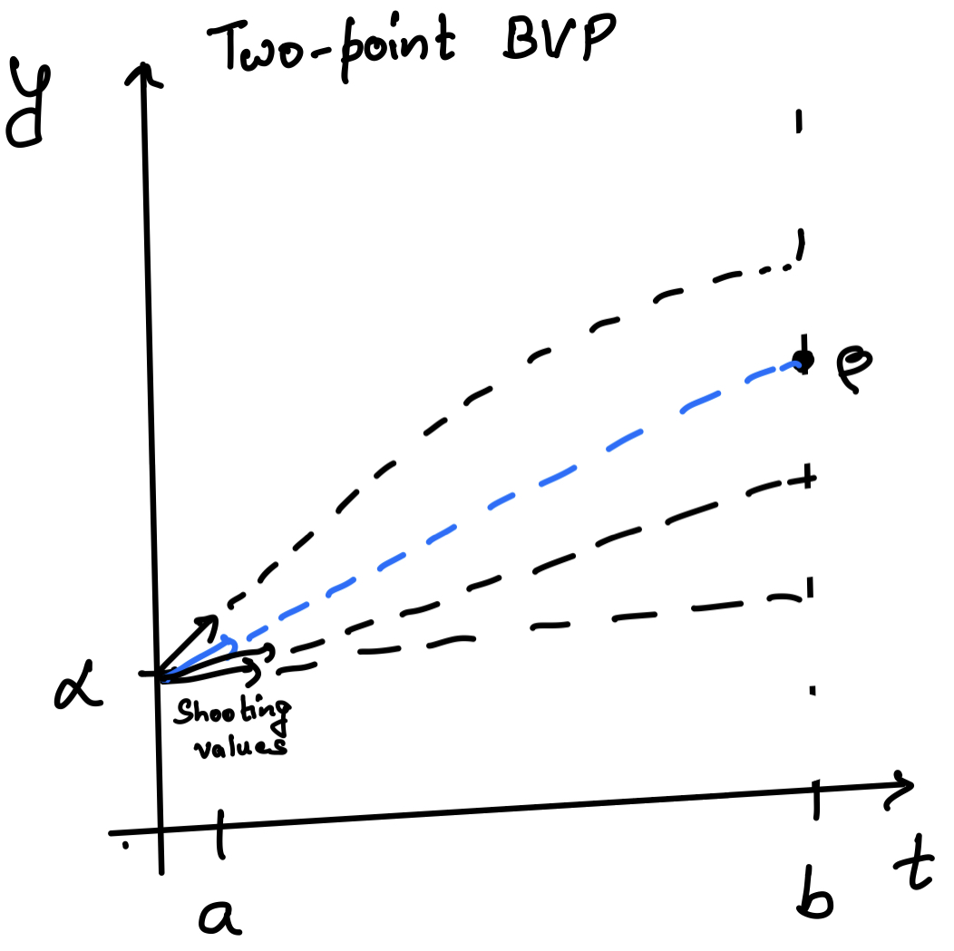
The value of $\kappa$ is the slope of the y function at $t=a$.
The shooting method gives a procedure to iteratively determine this constant $\kappa$. In other words, we will be applying our modified initial value problem approach (the Runge-Kutta method) to solve the boundary value problems.
Quick check: In the shooting method, what role does the function $F(\kappa) = y(b) - \beta$ play?
Example 1
Let us start with a very simple problem of freefall of a ball under the effect of gravity.
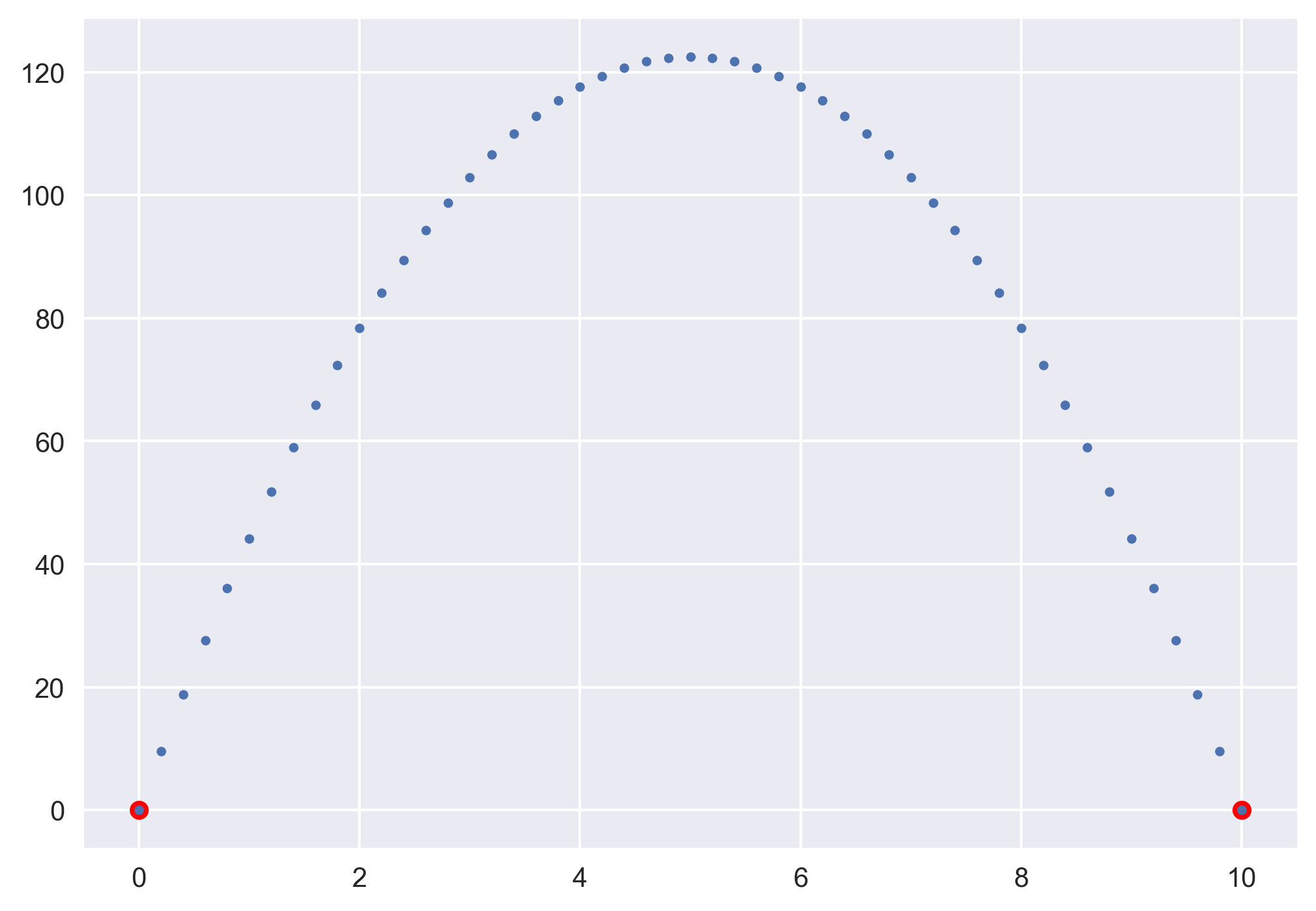
\[\frac{d^2\vec{y}}{dt^2} = -g\]where, $g=9.8$ m/s^2. The boundary condition here is that we start at $y=0$ with unknown velocity, but we know that it will be back at $t=10$.
import numpy as np
from scipy.integrate import solve_ivp
from scipy import optimize
import matplotlib.pyplot as plt
plt.style.use('seaborn')

g = 9.8
y0 = 0
tf = 10


def f(t, r):
    y, v = r
    dy_dt = v  # velocity
    d2y_dt2 = -g  # acceleration

    return dy_dt, d2y_dt2


@np.vectorize
def shooting_eval(v0):
    sol = solve_ivp(f, (t[0], t[-1]), (y0, v0), t_eval=t)
    y_num, v = sol.y
    return y_num[-1]


v0 = 60  # guess the initial velocity
t = np.linspace(0, tf, 51)

fig, ax = plt.subplots()
v0 = np.linspace(0, 100, 100)
plt.plot(v0, shooting_eval(v0), label='Shooting evaluation')
plt.axhline(c="k")


# root finding: secant method (kind of Newton Raphson method where slope is unknown)
# Find a zero of the function func given a nearby starting point x0
v0 = optimize.newton(shooting_eval, 50)
print(v0)
plt.plot(v0, 0, 'ro', label=f'Solution: {v0:.1f}')

plt.grid(True)
plt.legend()
ax.set_xlabel('t')
ax.set_ylabel('y')
plt.savefig('example1_solution.png', bbox_inches='tight', dpi=300)
plt.close()
How optimize.newton does the “shooting” here. shooting_eval(v0) is the miss function $F$: it integrates the trajectory for a given launch velocity and returns the final height. Passing it to optimize.newton without a derivative makes SciPy use the secant method — it tries two nearby velocities, sees how the miss changes, and homes in on the v0 where the ball lands exactly at the target. That’s the whole shooting loop in one call.
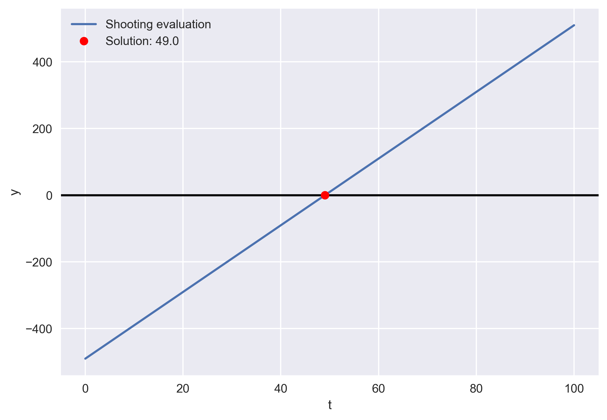
Here, we found the initial velocity to be 49.0 m/s.
# Plot the path

t = np. linspace(0, tf, 51)
sol = solve_ivp(f, (0, tf), (y0, v0), t_eval=t)
y, v = sol.y

plt.plot(t[0], y0, 'ro', label=f'Solution: {v0:.1f}')
plt.plot(t[-1], 0, 'ro', label=f'Solution: {v0:.1f}')
plt.plot(t, y, ".")

plt.savefig('example1_solution_path.png', bbox_inches='tight', dpi=300)
plt.close()
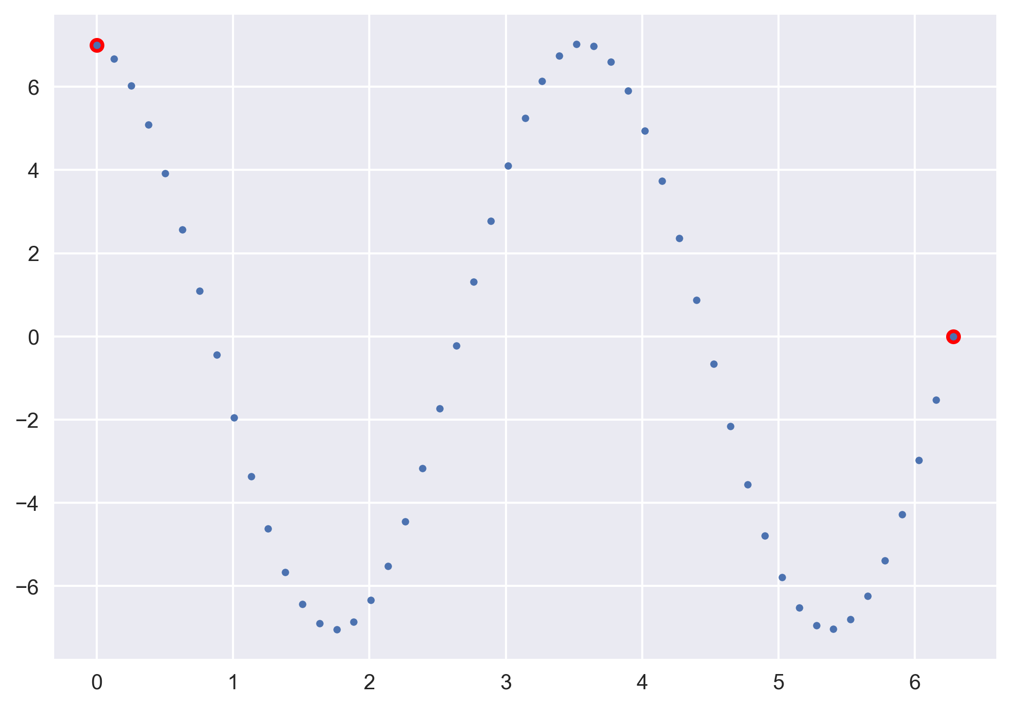
Example 2
Let us take another simple differential equation to solve.
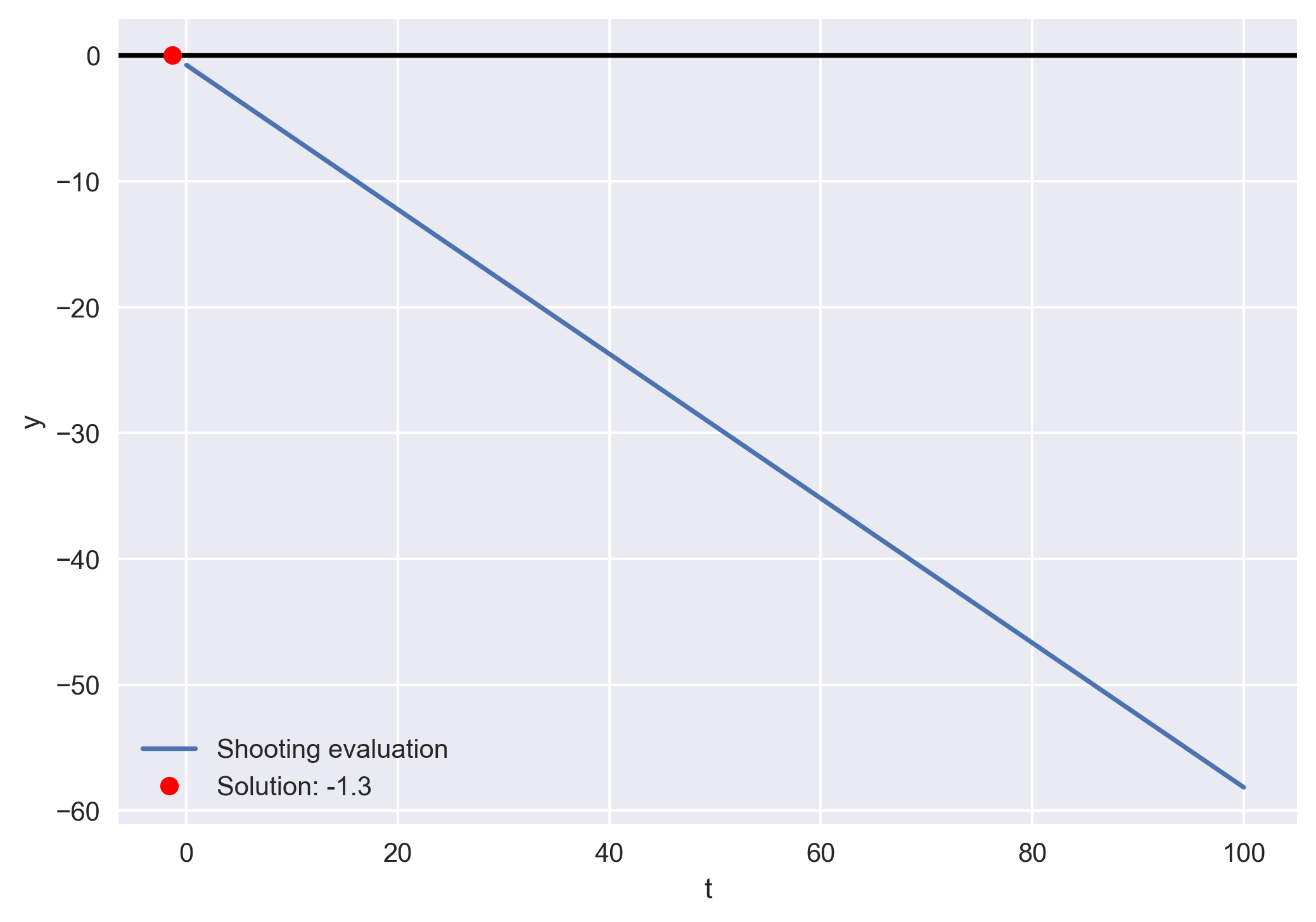
\[\frac{d^2\vec{y}}{dt^2} +3y = 0\]where, $y(0) = 7$ and $y(2*\pi)=0$.
import numpy as np
from scipy.integrate import solve_ivp
from scipy import optimize
import matplotlib.pyplot as plt
plt.style.use('seaborn')


# example d2y/dt2+3y = 0
# y(0) = 7 and y(2*pi)=0

y0 = 7
tf = 2 * np.pi


def f(t, r):
    y, v = r
    dy_dt = v  # velocity
    d2y_dt2 = -3 * y  # acceleration

    return dy_dt, d2y_dt2


@np.vectorize
def shooting_eval(v0):
    sol = solve_ivp(f, (t[0], t[-1]), (y0, v0), t_eval=t)
    y_num, v = sol.y
    return y_num[-1]


v0 = 60  # guess the initial velocity
t = np.linspace(0, 2 * np.pi, 100)

fig, ax = plt.subplots()
v0 = np.linspace(0, 100, 100)
plt.plot(v0, shooting_eval(v0), label='Shooting evaluation')
plt.axhline(c="k")


# root finding: secant method (kind of Newton Raphson method where slope is unknown)
# Find a zero of the function func given a nearby starting point x0
v0 = optimize.newton(shooting_eval, 50)
print(v0)
plt.plot(v0, 0, 'ro', label=f'Solution: {v0:.1f}')

plt.grid(True)
plt.legend()
ax.set_xlabel('t')
ax.set_ylabel('y')
plt.savefig('example2_solution.png', bbox_inches='tight', dpi=300)
plt.close()
# Plot the path

t = np. linspace(0, tf, 51)
sol = solve_ivp(f, (0, tf), (y0, v0), t_eval=t)
y, v = sol.y

plt.plot(t[0], y0, 'ro', label=f'Solution: {v0:.1f}')
plt.plot(t[-1], 0, 'ro', label=f'Solution: {v0:.1f}')
plt.plot(t, y, ".")

plt.savefig('example2_solution_path.png', bbox_inches='tight', dpi=300)
plt.close()
One update for a current SciPy/Matplotlib setup. plt.style.use('seaborn') was deprecated in Matplotlib 3.6 and removed in 3.8 — use plt.style.use('seaborn-v0_8') instead. Also note that scipy.integrate.solve_ivp is the modern replacement for the older odeint, and the code here already uses it. The rest runs unchanged.
Recap
- BVP → IVP + root find. The shooting method converts a two-endpoint problem into “guess the initial slope, integrate, correct.”
- The miss is a function of the guess. Define $F(\kappa) = y(b) - \beta$; the correct initial slope is the root $F(\kappa)=0$.
- Reduce order for the solver. Rewrite the 2nd-order ODE as two 1st-order equations ($y’ = z$, $z’ = f$) so
solve_ivpcan march it forward. - Let SciPy close the loop.
optimize.newtonon the miss function (no derivative → secant method) iterates the guess to convergence automatically.
Where to go next
scipy.integrate.solve_ivpdocs: docs.scipy.org/doc/scipy/reference/generated/scipy.integrate.solve_ivp.htmlscipy.optimize.newtondocs: docs.scipy.org/doc/scipy/reference/generated/scipy.optimize.newton.htmlscipy.integrate.solve_bvp(a dedicated BVP solver): docs.scipy.org/doc/scipy/reference/generated/scipy.integrate.solve_bvp.html- Related posts: Euler method · Runge–Kutta method · Newton–Raphson method
References
- Kutz, J. N. (2013). Data-driven modeling & scientific computation: methods for complex systems & big data. Oxford University Press.
Disclaimer of liability
The information provided by the Earth Inversion is made available for educational purposes only.
Whilst we endeavor to keep the information up-to-date and correct. Earth Inversion makes no representations or warranties of any kind, express or implied about the completeness, accuracy, reliability, suitability or availability with respect to the website or the information, products, services or related graphics content on the website for any purpose.
UNDER NO CIRCUMSTANCE SHALL WE HAVE ANY LIABILITY TO YOU FOR ANY LOSS OR DAMAGE OF ANY KIND INCURRED AS A RESULT OF THE USE OF THE SITE OR RELIANCE ON ANY INFORMATION PROVIDED ON THE SITE. ANY RELIANCE YOU PLACED ON SUCH MATERIAL IS THEREFORE STRICTLY AT YOUR OWN RISK.
Leave a comment