A quick look into the Sktime for time-series forecasting (codes included)
In this post, I will explore one of such Libraries that is rising real fast as a popular choice for Time series analysis in recent days - sktime. Sktime is a relatively new library in machine learning designed specifically for the time series. It is based on the scikit-learn library that I are familiar with but it has been tweaked for the time series. There are several approaches for machine learning in the Time series but the sktime takes a good bit from many different libraries and builds an efficient and compelling interface. So in my view, it could be a great starting point.
The goal is to try out several algorithms for forecasting time series using sktime.
Key idea — sktime gives forecasting a scikit-learn fit/predict interface, and can reduce it to plain regression. Every forecaster follows the same recipe: build it, fit(y_train), then predict(fh) for a forecasting horizon (the steps ahead you want). The clever part is reduction: a sliding window turns the series into supervised (X = last L values, y = next value) pairs, so any scikit-learn regressor (like KNeighborsRegressor) becomes a forecaster that predicts the horizon recursively. That unified interface lets you swap a naive baseline, exponential smoothing, and auto-ARIMA with one-line changes.
Install Sktime
Sktime has a good documentation for installation. The two approaches they suggest on their GitHub page are through pip and anaconda.
pip install sktime
I prefer the Anaconda way so I will use that but either way’s equally valid.
conda install -c conda-forge sktime
You may also need other libraries like matplotlib, seaborn,for running all the codes below.
You can simply install that by using the following command:
conda install -c conda-forge matplotlib seaborn
pip install pmdarima
Heads-up — sktime’s API has moved on since 2021. The code below is preserved as originally written, but a few calls no longer work on current sktime (0.20+). Here are the drop-in replacements:
smape_losswas removed. Replacefrom sktime.performance_metrics.forecasting import smape_lossandsmape_loss(y_pred, y_test)with the parametrized metric:from sktime.performance_metrics.forecasting import mean_absolute_percentage_error mean_absolute_percentage_error(y_test, y_pred, symmetric=True) # this is sMAPEReducedForecasterwas removed — use the factorymake_reduction(and drop thescitypeargument):from sktime.forecasting.compose import make_reduction forecaster = make_reduction(regressor, window_length=15, strategy="recursive")temporal_train_test_splitmoved tofrom sktime.split import temporal_train_test_split.
NaiveForecaster, ExponentialSmoothing, AutoARIMA, and load_airline still live at the same imports. The concepts — fit/predict, forecasting horizon, reduction — are unchanged.
Data: Airline dataset
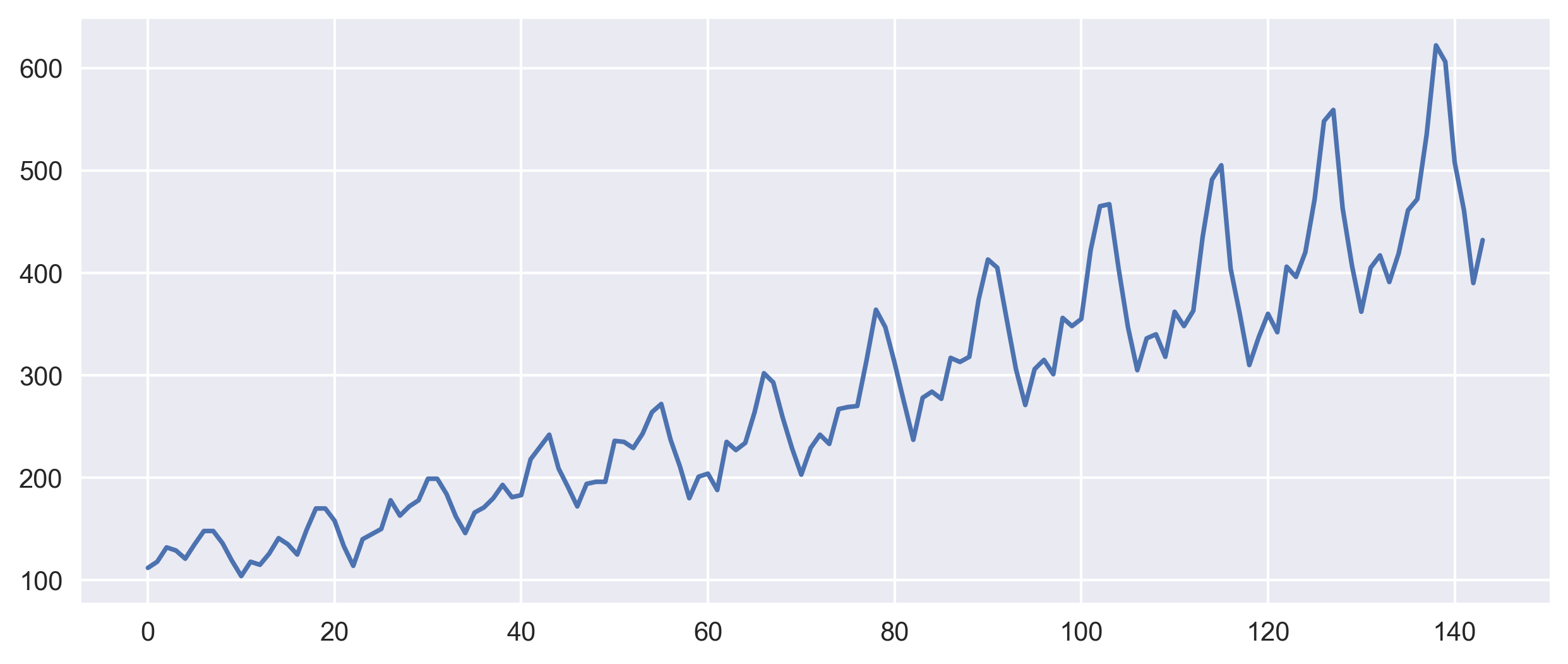
Let us first start with the data set that has become a standard for testing any subroutines in programming and data science. We will use the Box-Jenkins univariate airline data set, which shows the number of international airline passengers per month from 1949 - 1960. We use the exact dataset that has also been used by the Sktime documentation.
from sktime.datasets import load_airline
import matplotlib.pyplot as plt
y = load_airline() #y is pandas series object

fig, ax = plt.subplots(1, figsize=(10, 4))
ax.plot(y.values) #I convert that into numpy array
plt.savefig('airline-data-plot.png', dpi=300, bbox_inches='tight')
plt.close('all')
Now I perform the standard technique of splitting the data set into the training and test parts. The train part is used to build the model and the test part is used to “test” the result of training. Sktime provides a module to do that in an efficient way. This is based on the SKlearn module but has been a tweak to work specifically for time series.
from sktime.forecasting.model_selection import temporal_train_test_split
y_train, y_test = temporal_train_test_split(y, test_size=36)

fig, ax = plt.subplots(1,1, figsize=(10, 4))
y_train.plot(ax=ax, label='y_train')
y_test.plot(ax=ax, label='y_test')
plt.legend()
plt.savefig('train-test-airline-data-plot.png', dpi=300, bbox_inches='tight')
plt.close('all')
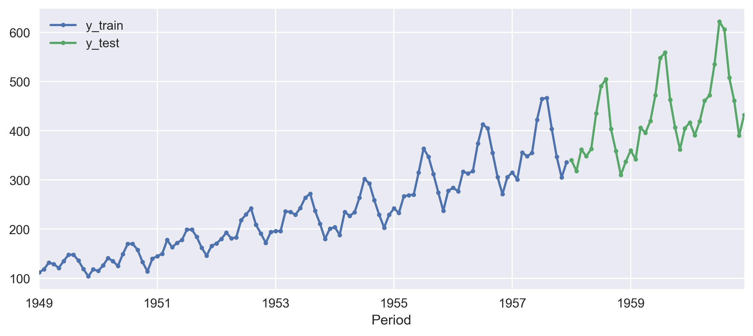
Here, I will try to predict the last 3 years of data (hence the test size of 12*3 = 36), using the previous years as training data.
Analysis
Now, I need to generate a forecasting horizon to use in the algorithm for forecasting. For this case, I’re interested in predicting from the first to the 36th step ahead because I used 36 data points as our test part.
import numpy as np
fh = np.arange(len(y_test)) + 1  # forecasting horizon
Similar to many other machine learning modules, in order to make forecasts, I need to first build a model, then fit it to the training data, and finally call predict to generate forecasts for the given forecasting horizon.
NaiveForecaster
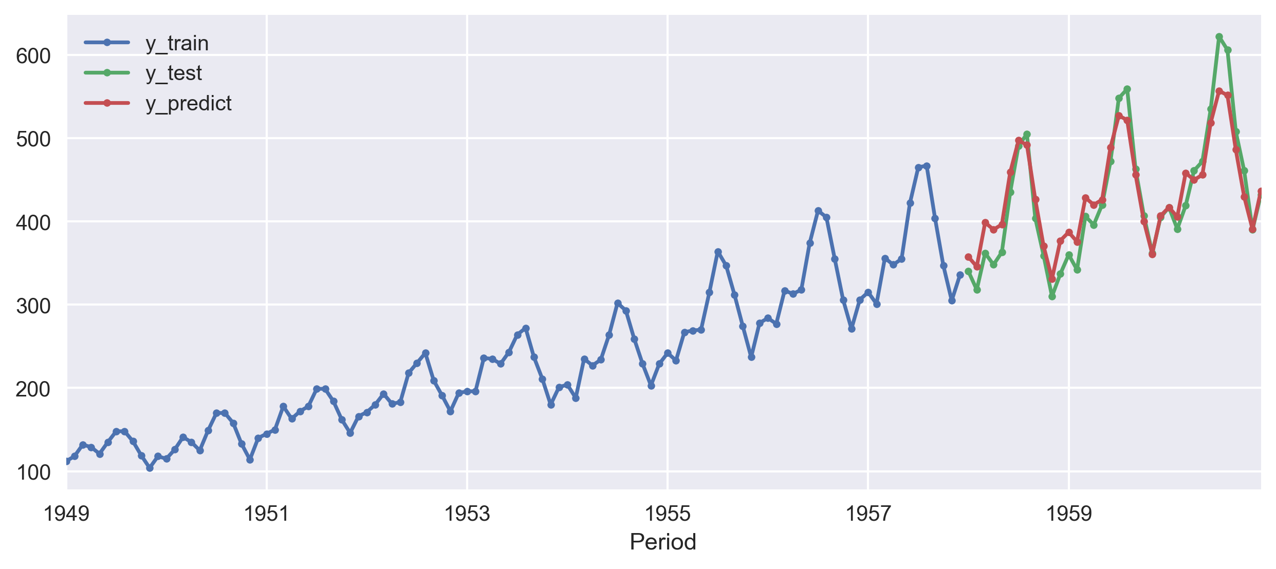
We will use NaiveForecaster to make forecasts using simple strategies.
from sktime.forecasting.naive import NaiveForecaster
from sktime.performance_metrics.forecasting import smape_loss

forecaster = NaiveForecaster(strategy="last", sp=12)
forecaster.fit(y_train)
y_pred = forecaster.predict(fh)
print(smape_loss(y_pred, y_test))

fig, ax = plt.subplots(1, 1, figsize=(10, 4))
y_train.plot(ax=ax, label='y_train', style='.-')
y_test.plot(ax=ax, label='y_test', style='.-')
y_pred.plot(ax=ax, label='y_predict', style='.-')
plt.legend()
plt.savefig('predict-airline-data-plot.png', dpi=300, bbox_inches='tight')
plt.close('all')
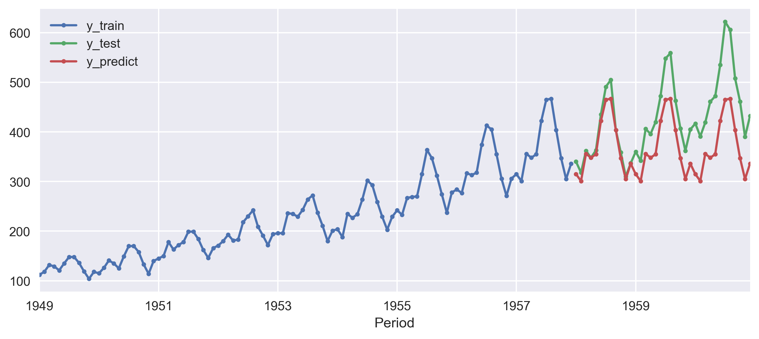
In the above code, I chose the strategy for the forecast to be last, and seasonal periodicity of 12. Also, I used the sMAPE (symmetric mean absolute percentage error) to quantify the accuracy of our forecasts. A lower sMAPE means higher accuracy.
There are other popular performance evaluation metrics available for regression problems such as Mean Absolute Percentage Error (MAPE), Mean Absolute Scaled Error (MASE), Mean Directional Accuracy (MDA), etc, and I will investigate them in future posts. The other available strategies are drift and mean but since our data has an increasing trend so those may not be a good strategy.
In this case, I get the smape_loss to be 0.1454 for the last strategy but if I use mean then the prediction will go worse and I can see that reflected from the smape_loss value of 0.5908.
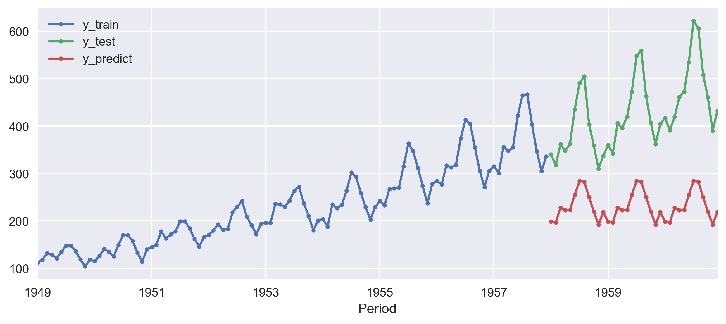
smape_loss is 0.5908KNeighborsRegressor
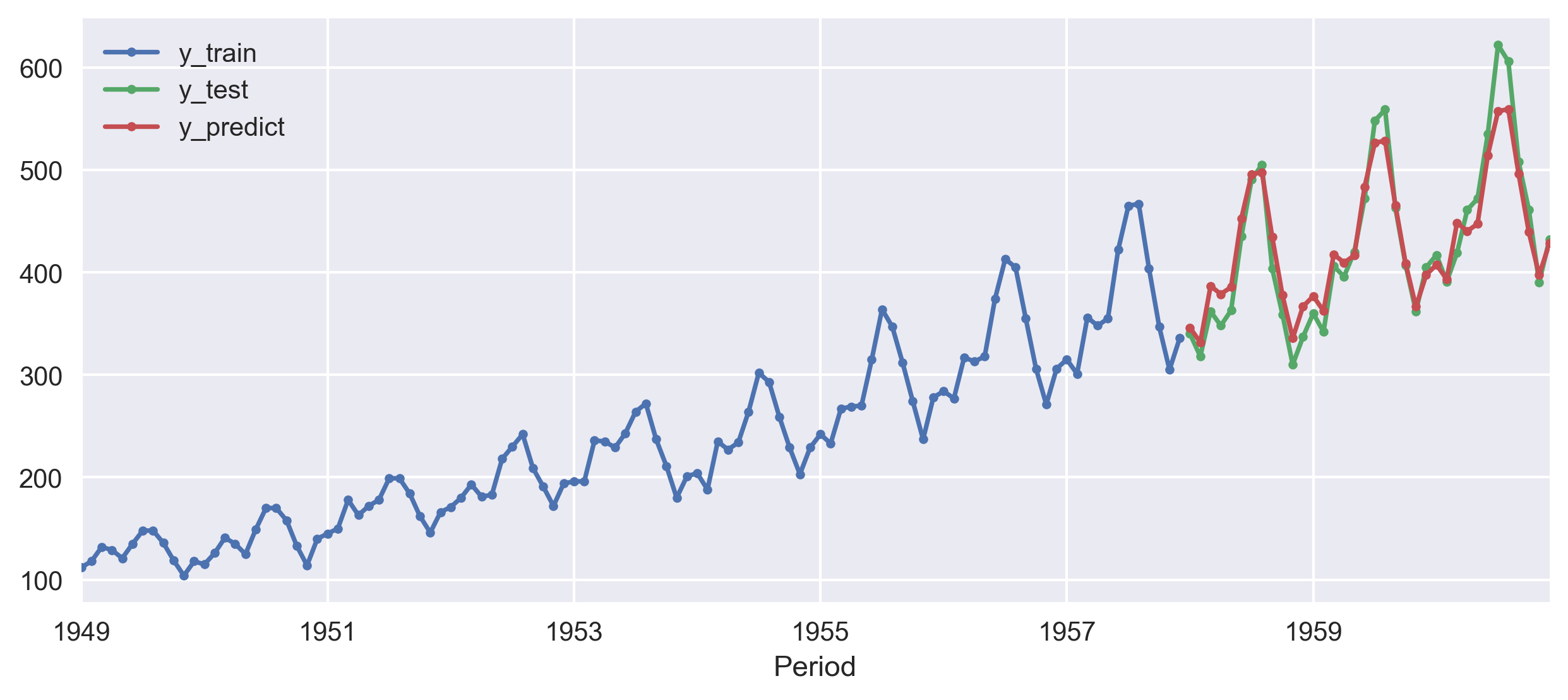
Now, let us use the regression based on k-nearest neighbors to forecast the time series. Here, I use the KNeighborsRegressor from the scikit-learn library. This predicts the target by local interpolation of the targets associated of the nearest neighbors in the training set.
from sktime.forecasting.compose import ReducedForecaster
from sklearn.neighbors import KNeighborsRegressor

regressor = KNeighborsRegressor(n_neighbors=1)
forecaster = ReducedForecaster(
    regressor, scitype="regressor", window_length=15, strategy="recursive"
)
forecaster.fit(y_train)
y_pred = forecaster.predict(fh)
print(smape_loss(y_test, y_pred))

fig, ax = plt.subplots(1, 1, figsize=(10, 4))
y_train.plot(ax=ax, label='y_train', style='.-')
y_test.plot(ax=ax, label='y_test', style='.-')
y_pred.plot(ax=ax, label='y_predict', style='.-')
plt.legend()
plt.savefig('predict-KNeighborsRegressor-airline-data-plot.png',
            dpi=300, bbox_inches='tight')
plt.close('all')

smape_loss in this case is 0.1418The smape_loss, in this case, is 0.1418. We got a slight improvement from the NaiveForecaster but the difference is not substantial.
Quick check: How does a KNeighborsRegressor (a plain scikit-learn regressor) end up forecasting a time series here?
Statistical forecasters
sktime also offers a number of statistical forecasting algorithms, based on implementations in statsmodels. We can then specify exponential smoothing with an additive trend component and multiplicative seasonality.
from sktime.forecasting.exp_smoothing import ExponentialSmoothing

forecaster = ExponentialSmoothing(trend="add", seasonal="additive", sp=12)
forecaster.fit(y_train)
y_pred = forecaster.predict(fh)
print(smape_loss(y_test, y_pred))

fig, ax = plt.subplots(1, 1, figsize=(10, 4))
y_train.plot(ax=ax, label='y_train', style='.-')
y_test.plot(ax=ax, label='y_test', style='.-')
y_pred.plot(ax=ax, label='y_predict', style='.-')
plt.legend()
plt.savefig('predict-ExponentialSmoothing-airline-data-plot.png',
            dpi=300, bbox_inches='tight')
plt.close('all')
smape_loss in this case is 0.0502.Auto selected best ARIMA model
Sktime interfaces with pmdarima, a package for automatically selecting the best ARIMA model. This since searches over a number of possible model parametrizations, it is usually a bit slow.
from sktime.forecasting.arima import AutoARIMA

forecaster = AutoARIMA(sp=12, suppress_warnings=True)
forecaster.fit(y_train)
y_pred = forecaster.predict(fh)
print(smape_loss(y_test, y_pred))

fig, ax = plt.subplots(1, 1, figsize=(10, 4))
y_train.plot(ax=ax, label='y_train', style='.-')
y_test.plot(ax=ax, label='y_test', style='.-')
y_pred.plot(ax=ax, label='y_predict', style='.-')
plt.legend()
plt.savefig('predict-AutoARIMA-airline-data-plot.png',
            dpi=300, bbox_inches='tight')
plt.close('all')
smape_loss in this case is 0.0411.Conclusions
Sktime is a promising library for machine learning applications for time series and has advantages over using lower-level libraries such as Sklearn. Also, as it interfaces with several other mature machine learning libraries in Python, it can be used to efficiently employ algorithms from sklearn or pmdarima directly for the time series analysis.
This tutorial is simple in nature and the future posts will cover the advanced applications of sktime as I get more into it. Sktime also has a powerful library for univariate time series classification analysis. We will cover that in future posts.
Also, I will look into the other popular libraries for time series analysis such as tslearn (for classification/clustering), pyts (for classification), statmodels (forecasting and time series analysis), gluon-ts (forecasting, anomaly detection), tsfresh (feature extraction), etc.
Recap
- One interface, many models. Every sktime forecaster uses
fit(y_train)thenpredict(fh); swapNaiveForecaster,ExponentialSmoothing,AutoARIMA, or a reduced regressor with a one-line change. - The forecasting horizon
fhsays how many steps ahead to predict (here1…36, the 3-year test window). - Reduction = forecasting via regression.
make_reduction(formerlyReducedForecaster) slides a window to build(X, y)pairs so any sklearn regressor forecasts recursively. - Score with sMAPE. Lower is better; on this data AutoARIMA (0.041) beat ExponentialSmoothing (0.050), KNN (0.142), and the naive baseline (0.145).
- Update the imports. On current sktime use
mean_absolute_percentage_error(..., symmetric=True),make_reduction, andsktime.split.
Where to go next
- sktime forecasting tutorial (official): sktime.net — forecasting
make_reductiondocs: sktime.net — make_reduction
References
- sktime: A Unified Interface for Machine Learning with Time Series — Löning, M., Bagnall, A., Ganesh, S., Kazakov, V., Lines, J., & Király, F. J., 2019, Workshop on Systems for ML at NeurIPS 2019 (arXiv:1909.07872).
- Forecasting with sktime (official tutorial)
Disclaimer of liability
The information provided by the Earth Inversion is made available for educational purposes only.
Whilst we endeavor to keep the information up-to-date and correct. Earth Inversion makes no representations or warranties of any kind, express or implied about the completeness, accuracy, reliability, suitability or availability with respect to the website or the information, products, services or related graphics content on the website for any purpose.
UNDER NO CIRCUMSTANCE SHALL WE HAVE ANY LIABILITY TO YOU FOR ANY LOSS OR DAMAGE OF ANY KIND INCURRED AS A RESULT OF THE USE OF THE SITE OR RELIANCE ON ANY INFORMATION PROVIDED ON THE SITE. ANY RELIANCE YOU PLACED ON SUCH MATERIAL IS THEREFORE STRICTLY AT YOUR OWN RISK.
Leave a comment