Autoencoders for Seismic Waveforms: Compress, Learn, and Generate
Loading likes…
A seismic waveform is a dense record of ground motion: often one or three components, thousands of samples, and a mixture of arrivals, coda, noise, instrument response, and path effects. An autoencoder turns that complexity into a practical learning problem: compress the waveform into a latent representation, then reconstruct it well enough that the representation still carries useful structure.
That single idea reaches well beyond compression: it supports denoising, quality control, similarity search, and feature transfer, and its generative variants now show up in ground-motion generation and inversion workflows. In this post, I start with the basic autoencoder, build a small synthetic denoising experiment to make the idea concrete, and then follow it into current seismological applications.
The key idea
An autoencoder usually learns a representation without requiring a human label for every waveform. Its reconstruction target comes from the waveform itself, or from an uncorrupted counterpart in a denoising task. Whether that representation is actually useful is a separate question, and we still have to test it against the real scientific or operational task.
Start with a waveform and keep only what matters
Let $\mathbf{x}$ be a waveform window or a spectrogram. An encoder converts it to a latent vector $\mathbf{z}$, and a decoder converts that vector back to a reconstruction $\hat{\mathbf{x}}$:
The encoder is a learned compressor; the decoder is a learned decompressor. Training adjusts both so that the reconstruction resembles the input. Hinton and Salakhutdinov (2006) showed that a network can learn nonlinear, low-dimensional codes by reconstructing high-dimensional data.
Figure 1 separates the encoder–decoder training pathway from the downstream uses of the latent code.
A small reconstruction error is only the beginning
The simplest objective is a reconstruction loss:
Minimizing this loss teaches the model one thing: make its output resemble its input. In an undercomplete autoencoder, the latent vector has fewer numbers than the waveform. The network cannot carry every sample through unchanged, so it must encode patterns that recur in the training data, such as pulse shape, coda, or typical noise structure. That is where compression comes from.
An overcomplete autoencoder has a latent vector at least as large as its input. It can still learn a useful representation, but it also has enough capacity to learn an unhelpful near-copy of the input. It therefore needs another constraint: for example, reconstruct a clean waveform from a corrupted input, mask part of the input, penalize the code, or restrict the architecture. These constraints make copying harder and reward structure that generalizes beyond one trace.
The limitation is just as important: low reconstruction error does not prove that the model preserved the feature that matters. An autoencoder can reproduce broad waveform shape while softening a subtle onset, altering amplitude relationships, or learning an instrument-specific shortcut. Kong et al. (2021) tested whether an autoencoder trained on earthquake waveforms could provide reusable features for event discrimination and phase picking. The transferred encoder was helpful only when the downstream task needed similar features and the model design and training strategy matched the task; a comparable model trained directly for that task was often stronger. The lesson I take from this: test transfer against a task-specific baseline rather than assuming a good reconstruction is a good feature set.
What does a small reconstruction error establish?
Four common forms of the same idea
The word autoencoder describes the encoder–decoder idea, not one fixed architecture. Choose the training target to match the problem.
| Form | What changes | Useful when… |
|---|---|---|
| Undercomplete AE | Reconstructs the input through a smaller latent code | Compressing or representing a consistently processed waveform archive |
| Denoising AE | Reconstructs an uncorrupted target from a corrupted input | Learning features less sensitive to a specified corruption process |
| Convolutional AE | Uses convolutional layers; it can still be standard, denoising, or variational | Working with local patterns in time series or time–frequency representations |
| Variational AE (VAE) | Learns a latent distribution and regularizes it toward a prior | Sampling from a structured latent space or defining a learned prior |
The denoising version is especially intuitive for seismology. Corrupt a waveform during training, then ask the model to recover its uncorrupted counterpart. Vincent et al. (2008) partially corrupted each training pattern and trained the network to reconstruct the original pattern, encouraging representations that are robust to the chosen corruption. Because an individual input value may be missing or unreliable, the hidden code has to use relationships among values rather than simply copy them; for a waveform, that means using temporal context.
A short detour: how does a VAE make a sampleable latent space?
A VAE is an autoencoder with one deliberate change: the encoder does not return one fixed code. For each input waveform, it returns the center and spread of a small Gaussian cloud in latent space:
Here, $\boldsymbol{\mu}$ says where the waveform belongs in latent space and $\boldsymbol{\sigma}$ says how wide its local cloud is. The decoder receives a sample from that cloud, not just its center. During training, draw that sample as
then decode $\mathbf{z}$ back to $\hat{\mathbf{x}}$. Writing the sample this way is the reparameterization trick: the random draw is isolated in $\boldsymbol{\epsilon}$, so gradients can still update $\boldsymbol{\mu}$ and $\boldsymbol{\sigma}$. Kingma and Welling (2014) introduced this trainable construction.
The VAE loss has two jobs:
The first term prevents the decoder from forgetting the waveform. The Kullback–Leibler (KL) divergence measures how different this waveform’s latent Gaussian is from the chosen prior $\mathcal{N}(\mathbf{0},\mathbf{I})$. For the diagonal Gaussian above, it penalizes latent means far from zero and variances far from one. It is zero only when the two distributions match. In plain language: reconstruction keeps each waveform recognizable; KL prevents every waveform from claiming an isolated, incompatible patch of latent space.
After training, this shared map is what makes generation possible. Sample $\mathbf{z}\sim\mathcal{N}(\mathbf{0},\mathbf{I})$ and pass it through the decoder; unlike a standard autoencoder, the decoder has been trained to see latent samples from roughly that region. The learned $\boldsymbol{\sigma}$ is a latent-space scale, however—not automatically a calibrated uncertainty on a phase pick, source parameter, or ground-motion prediction.
Use this extension when variation is part of the question: generating a family of plausible ground motions for one scenario, or representing several subsurface models that fit the same observations. It is not automatically better for ordinary compression; its regularization trades some reconstruction detail for a more structured, sampleable latent space.
A controlled synthetic denoising experiment
To see all of this working, I built a small denoising experiment from scratch. I generate single-component synthetic waveform windows with 256 samples at 50 Hz, giving a duration of 5.12 s. Every clean window contains an early Ricker pulse with a central frequency between 6 and 8 Hz followed by a damped sinusoidal coda, and half of the windows also contain a later, lower-frequency Ricker pulse and coda. I refer to these two groups below as the early-pulse-only and early-and-late-pulse families.
To be clear about what these signals are: morphological test signals, not P and S arrivals calculated from a source model, velocity structure, or propagation path. I corrupt each clean waveform with correlated Gaussian noise plus additive white Gaussian noise. That corruption is useful precisely because it is controlled, but it does not reproduce the full nonstationary and site-dependent character of real seismic noise.
I train on 900 independently generated windows and evaluate on 240 additional windows drawn from the same parameter ranges. The model is a dense undercomplete autoencoder with layer widths 256 → 64 → 8 → 64 → 256. I give additional weight in the loss to samples with larger target amplitudes so that the near-zero parts of the windows do not dominate optimization.
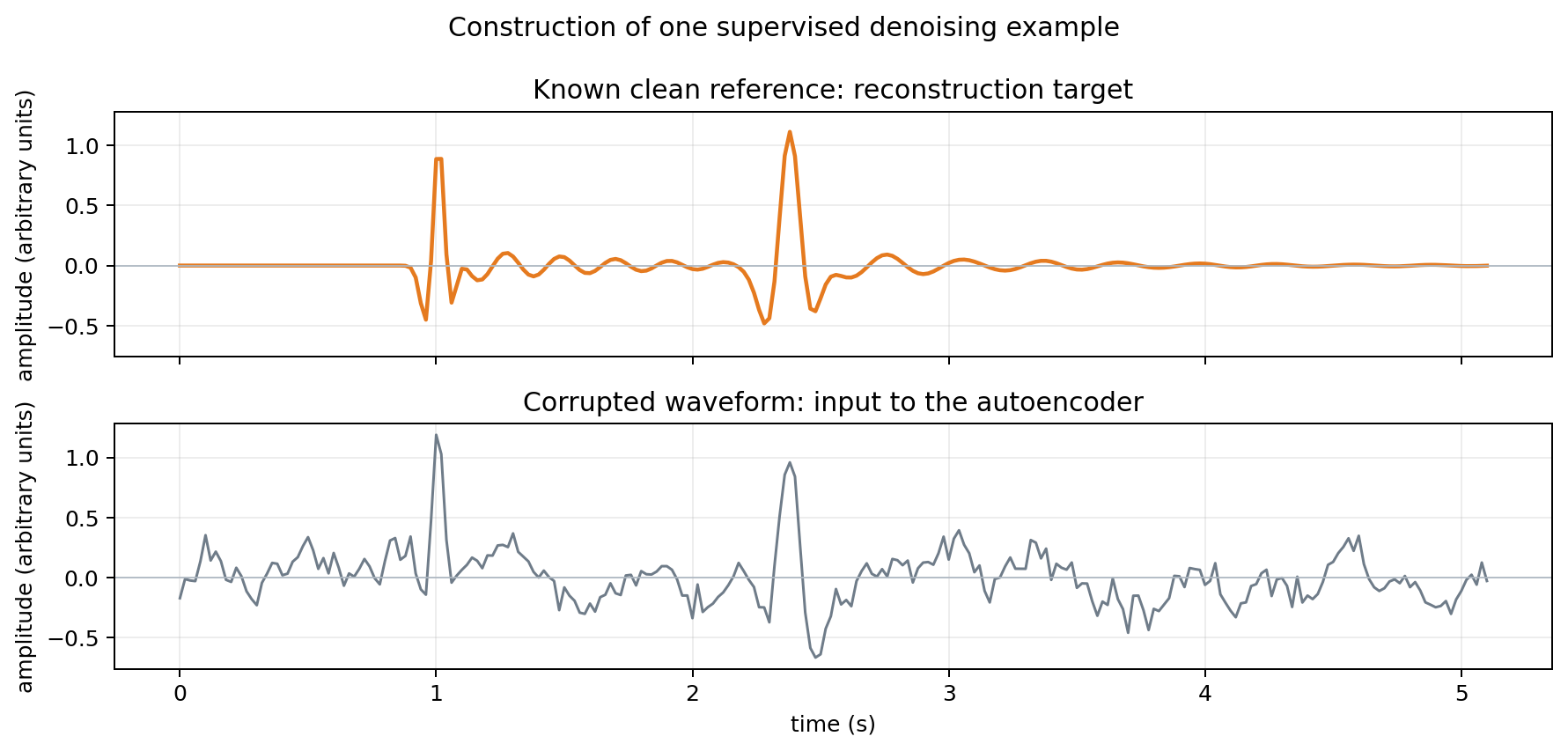
In Figure 2, the upper trace is the reconstruction target and the lower trace is the corrupted input. At inference time, the encoder sees only the corrupted waveform; I keep the clean waveform solely to train the denoising objective and to quantify reconstruction error.
I train the model in a supervised denoising configuration: noisy is the input and clean is the target, rather than the input reconstructing itself:
def noisy_waveform(rng, clean):
    correlated = np.convolve(
        rng.normal(size=N_SAMPLES), np.ones(9) / 9, mode="same"
    )
    correlated /= np.std(correlated) + 1e-8
    return (
        clean
        + rng.uniform(0.12, 0.24) * correlated
        + rng.uniform(0.03, 0.09) * rng.normal(size=N_SAMPLES)
    )

train_x, train_y, _ = dataset(rng, 900)  # noisy inputs, clean targets
test_x, test_y, labels = dataset(rng, 240)

for _ in range(700):
    order = rng.permutation(len(train_x))
    for start in range(0, len(order), 64):
        batch = order[start:start + 64]
        loss, gradients = model.gradients(train_x[batch], train_y[batch])
        model.update(gradients)
I implemented everything in NumPy, with a hyperbolic-tangent activation in the hidden layers, Adam optimization, and a fixed random seed so that the figures and numerical values here are reproducible.
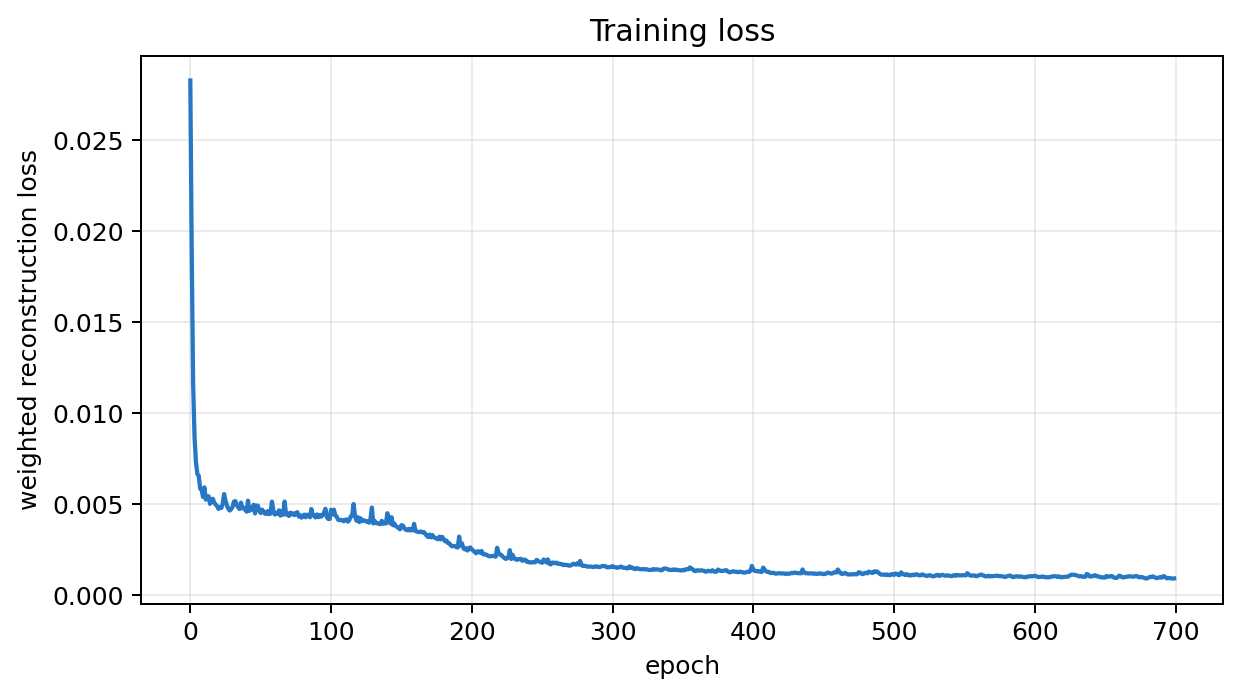
Figure 3 shows that the weighted training objective converges. It says nothing about generalization, because the curve is calculated from the training set, so Figures 4–7 use the separate set of 240 synthetic test windows.
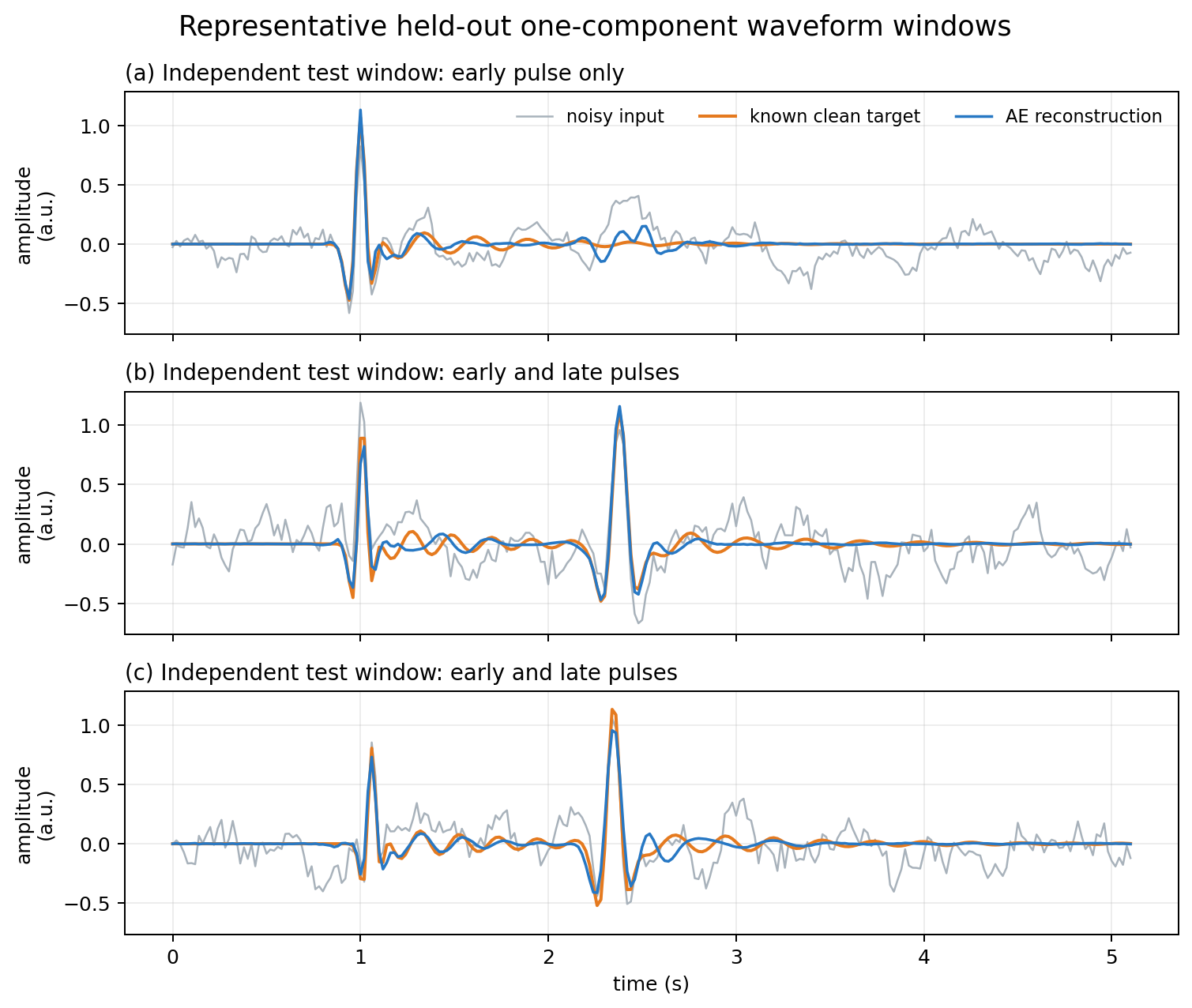
Each row in Figure 4 is one independently generated waveform window. Panel (a) illustrates the early-pulse-only family; panels (b) and (c) show two realizations from the early-and-late-pulse family. The reconstruction suppresses much of the imposed background noise and retains the dominant pulse timing. It also smooths some coda oscillations and does not reproduce every target amplitude exactly.
Across all samples in the fixed test set, the noisy inputs have a mean-squared error (MSE) of $0.0388$ relative to the clean targets. The reconstruction MSE is $0.00462$, corresponding to an $88.1\%$ reduction:
I would not read this as an expected denoising improvement for field recordings. It describes an in-distribution synthetic test: the training and test windows were generated by the same signal and noise models.
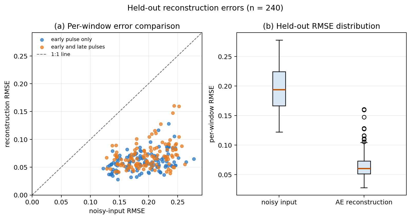
All 240 windows in this test realization fall below the 1:1 line in Figure 5a. The median per-window root-mean-square error (RMSE) decreases from $0.194$ for the noisy inputs to $0.0607$ for the reconstructions. Figure 5b also shows several reconstruction outliers, which are obscured by the aggregate MSE.
These statistics are descriptive rather than an uncertainty analysis: the experiment uses one random seed and one synthetic test distribution. For field data, I would separate training and testing by event where possible, and stratify performance by station, component, signal-to-noise ratio, magnitude, distance, phase window, and time period. Randomly splitting highly related windows from the same event between training and testing can otherwise produce an optimistic result.
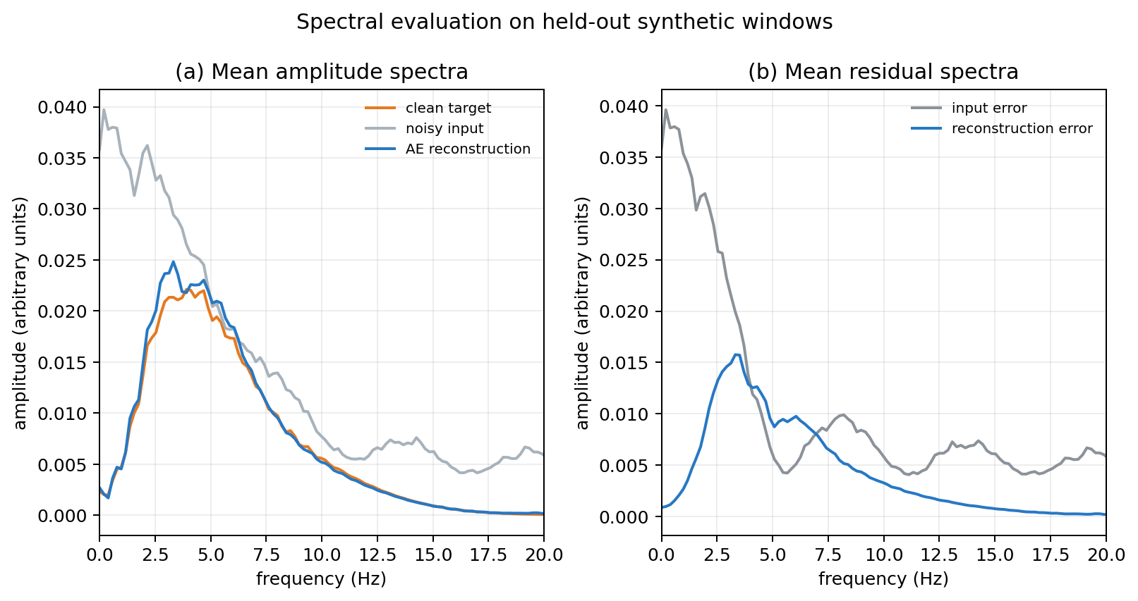
Figure 6a shows that the mean reconstruction spectrum follows the clean target more closely than the noisy input over much of the plotted band. The residual comparison in Figure 6b is more informative: reconstruction strongly reduces the low-frequency and high-frequency components of the imposed noise, but the reconstruction residual is locally comparable to, or larger than, the input residual at approximately 3.5–5.5 Hz. This indicates model error within part of the signal band, consistent with the smoothing and amplitude differences visible in Figure 4.
Mean amplitude spectra do not measure phase fidelity, arrival-time bias, or variability among individual windows. For field data, I would repeat the spectral evaluation by station, component, phase window, and frequency band, with consistent physical units and preprocessing, and match the metric to the intended downstream measurement.
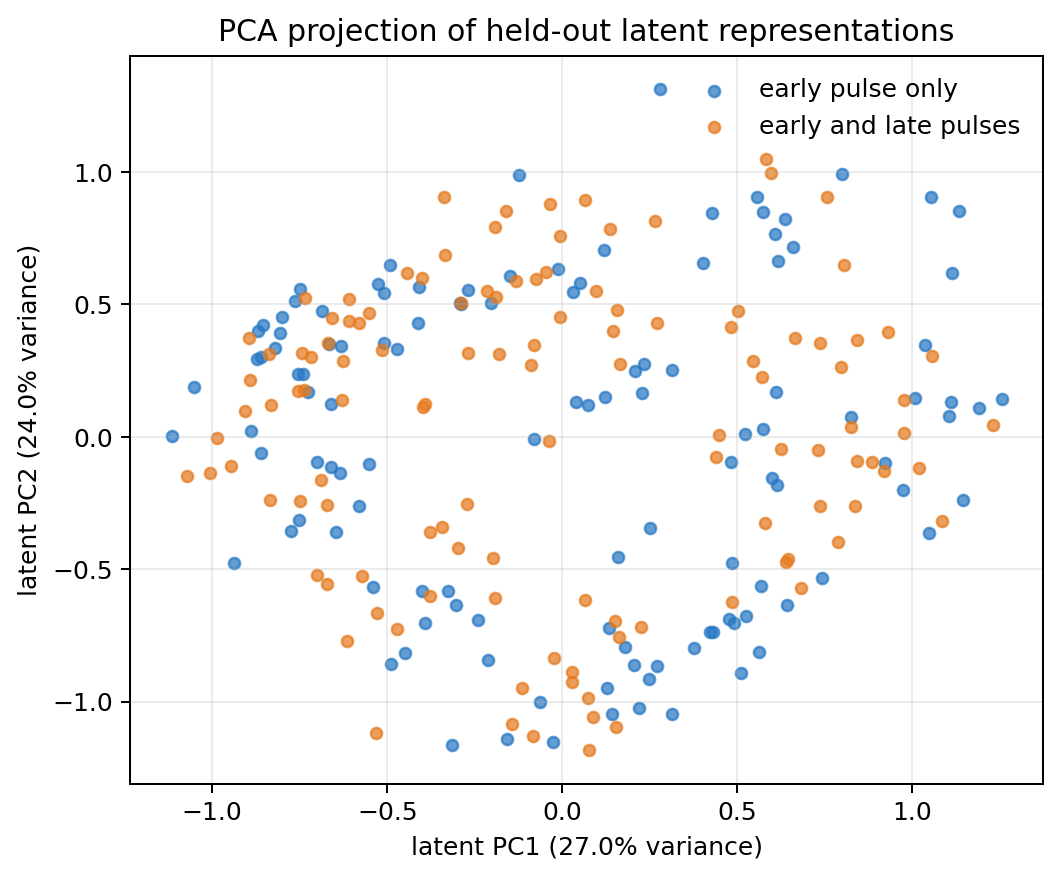
Rather than plotting an arbitrary pair of latent coordinates, Figure 7 shows a principal-component analysis (PCA) of all eight latent variables. The first two principal components account for $51.0\%$ of the latent variance, and the early-pulse-only and early-and-late-pulse windows overlap substantially.
This result is still informative even though it does not show two compact clusters. The autoencoder was optimized to reconstruct clean waveforms, not to separate the two families or make Euclidean latent distance correspond to waveform similarity. A two-dimensional PCA projection can also hide structure present in the remaining latent dimensions. Consequently, a visually organized latent plot is neither necessary nor sufficient evidence that the representation supports classification, clustering, or template matching. Those claims require task-specific, held-out tests.
Applications in seismic waveform analysis
Waveform similarity and template matching. Within a consistently processed archive, seismograms occupy a constrained part of all possible time series. Valentine and Trampert (2012) used autoencoders for data-space reduction, quality assessment, and searching of seismograms. A compact code can make similarity search and clustering more manageable than comparing every raw sample against every other trace.
For repeated-event detection or waveform template matching, an undercomplete or denoising autoencoder is generally a more direct starting point than a VAE because the objective is a stable, compact representation rather than sampling new waveforms. The encoder can be used to retrieve a short list of candidate windows from a large archive. Normalized waveform cross-correlation or another established matched-filter statistic should remain the baseline and can be used to verify the retrieved candidates.
Reconstruction training alone does not guarantee that nearby latent vectors are the most similar waveforms for a seismological task, as Figure 7 illustrates. If latent distance is central to the application, I would train or fine-tune the encoder with an explicit metric-learning or contrastive objective and evaluate it using known event families. Relevant tests include retrieval precision and recall, sensitivity to small time shifts, station and component transfer, and comparison with cross-correlation at the same computational budget.
For compression, evaluate more than mean-squared error. Check phase timing, polarity, amplitude ratios, Fourier amplitude spectra, coda characteristics, and every measurement that will later be made from the reconstructed data. Preprocessing choices such as normalization can remove absolute-amplitude information before the model sees it.
Transfer to a downstream task. An encoder trained on a large waveform collection can feed a smaller task-specific head for event discrimination, phase detection, clustering, or regression. This is related to the current push toward reusable seismic representations, but pretraining alone does not make a model a foundation model. The evaluation remains practical: compare against a well-tuned local baseline on held-out data.
Laurenti et al. (2026) fine-tuned a pretrained audio-compression autoencoder on seismic waveforms and evaluated its encoder embeddings on foreshock/aftershock classification, ground-motion estimation for early warning, and phase detection. The useful lesson is not that reconstruction solves every task, but that a representation should be tested across relevant tasks and data distributions.
The Kong et al. (2021) result I mentioned earlier is the complementary caution: transferred autoencoder features helped only for particular combinations of pretraining data, architecture, and downstream task, and models trained directly for the target task often performed better. I treat autoencoder pretraining as a hypothesis to test, not as an automatic improvement.
Quality control and anomaly detection. If an autoencoder is trained on a well-defined population of ordinary waveforms, an unusual trace may reconstruct poorly or fall in a low-density region of latent space. That suggests a route to quality control and anomaly detection, provided the distance or density score is defined and calibrated.
However, “unusual” is not a scientific class. Seasonal noise, clipping, timing errors, an instrument replacement, a new station, or a different source and path distribution can all increase reconstruction error. I treat the score as a prioritization variable for review: measure its false-alarm rate across stations and operating conditions, and recalibrate thresholds when the acquisition system or data distribution changes.
Reconstruction error is not a diagnosis. It measures disagreement with the learned training distribution under a chosen loss. Station response, sampling rate, network geometry, source population, propagation path, and noise conditions can all change that disagreement.
VAEs for generation and inverse problems
Autoencoders become especially interesting when reconstruction is only one stage in a larger generative workflow.
Waveform generation. Palgunadi et al. (2025) used a convolutional VAE to compress seismic spectrograms, trained a conditional diffusion model in that latent space, then decoded generated samples and transformed them back to waveforms. Ren et al. (2026) used a conditional dynamic VAE framework to generate ground-motion time series from earthquake and station information. Both aim to represent conditional variability rather than predict one deterministic trace. Their outputs still need to be checked against the intensity measures, duration, spectra, and component relationships required by the intended application.
Geophysical inversion. Inverse problems are often non-unique: distinct subsurface models can explain the same observations. Lopez-Alvis et al. (2022) used a VAE to assemble spatial prior uncertainty for cross-borehole ground-penetrating-radar travel-time inversion. Rodriguez et al. (2023) used a multimodal VAE to represent several plausible solutions, their probability of occurrence, and uncertainty in a one-dimensional magnetotelluric inverse problem. These are broader geophysics examples, but the lesson carries to seismic inversion: a learned prior can reduce the effective model space while explicitly importing the assumptions represented in its training data.
A learned prior is limited by its training distribution. If the training ensemble omits a plausible geological structure, a VAE-based inversion may exclude it or represent it poorly. Prior sensitivity and independent geological or geophysical constraints remain essential.
Evaluation should follow the intended use
| If the goal is… | Test… | Do not rely only on… |
|---|---|---|
| Compression | phase timing, polarity, spectra, amplitudes, coda, and compression ratio | average reconstruction error |
| Waveform retrieval | precision, recall, event-level splits, and comparison with cross-correlation | visual separation in a latent plot |
| Feature transfer | held-out downstream performance against a task-specific baseline | reconstruction accuracy alone |
| Anomaly detection | false alarms across stations, time periods, and changing noise | one threshold from one dataset |
| Ground-motion generation | conditioning fidelity, diversity, intensity measures, duration, spectra, and component coherence | waveforms that merely look realistic |
| Inversion | data fit, prior sensitivity, coverage of plausible models, and independent constraints | a smooth or visually plausible result |
Autoencoders are a family of representation-learning models rather than a single seismological algorithm. The architecture, loss, preprocessing, and training distribution determine what the latent representation preserves. Its scientific value is established only by an out-of-sample evaluation designed for the intended measurement or decision.
Further reading
- Read the companion post on seismic foundation models for a broader view of reusable waveform representations.
- Explore the SeisBench documentation to see how waveform datasets and pretrained seismological models are packaged for comparison.
- For a broader field overview, read Machine Learning in Earthquake Seismology (Mousavi & Beroza, 2023).
References
Hinton, G. E., & Salakhutdinov, R. R. (2006). Reducing the dimensionality of data with neural networks. Science, 313(5786), 504–507. https://doi.org/10.1126/science.1127647
Kingma, D. P., & Welling, M. (2014). Auto-encoding variational Bayes. In 2nd International Conference on Learning Representations (ICLR 2014). https://arxiv.org/abs/1312.6114v9
Kong, Q., Chiang, A., Aguiar, A. C., Fernández-Godino, M. G., Myers, S. C., & Lucas, D. D. (2021). Deep convolutional autoencoders as generic feature extractors in seismological applications. Artificial Intelligence in Geosciences, 2, 96–106. https://doi.org/10.1016/j.aiig.2021.12.002
Laurenti, L., Johnson, C. W., Trappolini, D., Tinti, E., Galasso, F., & Marone, C. (2026). Testing audio compression autoencoders for seismology: Moving toward foundation models. Journal of Geophysical Research: Machine Learning and Computation, 3(1), Article e2025JH000787. https://doi.org/10.1029/2025JH000787
Lopez-Alvis, J., Nguyen, F., Looms, M. C., & Hermans, T. (2022). Geophysical inversion using a variational autoencoder to model an assembled spatial prior uncertainty. Journal of Geophysical Research: Solid Earth, 127(3), Article e2021JB022581. https://doi.org/10.1029/2021JB022581
Mousavi, S. M., & Beroza, G. C. (2023). Machine learning in earthquake seismology. Annual Review of Earth and Planetary Sciences, 51(1), 105–129. https://doi.org/10.1146/annurev-earth-071822-100323
Palgunadi, K. H., Bergmeister, A., Bosisio, A., Ermert, L. A., Koroni, M., Perraudin, N., Dirmeier, S., & Meier, M.-A. (2025). High resolution seismic waveform generation using denoising diffusion. Journal of Geophysical Research: Machine Learning and Computation, 2(4), Article e2025JH000862. https://doi.org/10.1029/2025JH000862
Ren, P., Nakata, R., Lacour, M., Naiman, I., Nakata, N., Song, J., Bi, Z., Malik, O. A., Morozov, D., Azencot, O., Erichson, N. B., & Mahoney, M. W. (2026). Learning earthquake ground motions via conditional generative modeling. Nature Communications, 17(1), Article 4021. https://doi.org/10.1038/s41467-026-70719-2
Rodriguez, O., Taylor, J. M., & Pardo, D. (2023). Multimodal variational autoencoder for inverse problems in geophysics: Application to a 1-D magnetotelluric problem. Geophysical Journal International, 235(3), 2598–2613. https://doi.org/10.1093/gji/ggad362
Valentine, A. P., & Trampert, J. (2012). Data space reduction, quality assessment and searching of seismograms: Autoencoder networks for waveform data. Geophysical Journal International, 189(2), 1183–1202. https://doi.org/10.1111/j.1365-246X.2012.05429.x
Vincent, P., Larochelle, H., Bengio, Y., & Manzagol, P.-A. (2008). Extracting and composing robust features with denoising autoencoders. In W. W. Cohen, A. McCallum, & S. T. Roweis (Eds.), Proceedings of the 25th International Conference on Machine Learning (pp. 1096–1103). Association for Computing Machinery. https://doi.org/10.1145/1390156.1390294
Found this article useful?
Loading likes…
Disclaimer of liability
The information provided by the Earth Inversion is made available for educational purposes only.
Whilst we endeavor to keep the information up-to-date and correct. Earth Inversion makes no representations or warranties of any kind, express or implied about the completeness, accuracy, reliability, suitability or availability with respect to the website or the information, products, services or related graphics content on the website for any purpose.
UNDER NO CIRCUMSTANCE SHALL WE HAVE ANY LIABILITY TO YOU FOR ANY LOSS OR DAMAGE OF ANY KIND INCURRED AS A RESULT OF THE USE OF THE SITE OR RELIANCE ON ANY INFORMATION PROVIDED ON THE SITE. ANY RELIANCE YOU PLACED ON SUCH MATERIAL IS THEREFORE STRICTLY AT YOUR OWN RISK.
Leave a comment