Genetic Algorithm: a highly robust inversion scheme for geophysical applications
![]()
What is Optimization?
- “ The selection of a best element (with regard to some criteria) from some set of available alternatives” {Source: Wikipedia}
- Picking the “best” option from several ways of accomplishing the same task.
- We require a model which can give us the best result.
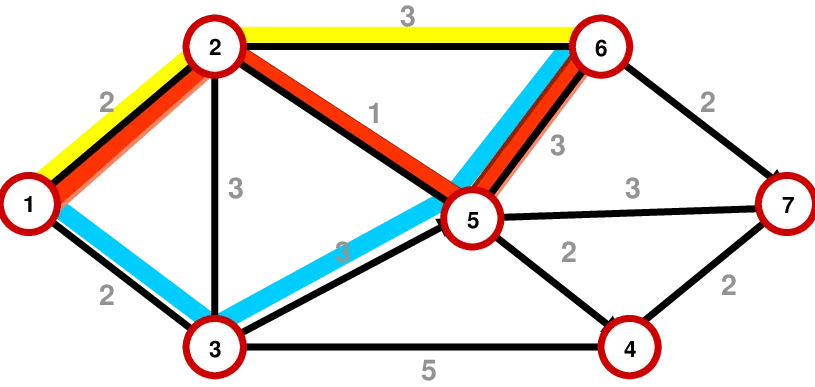
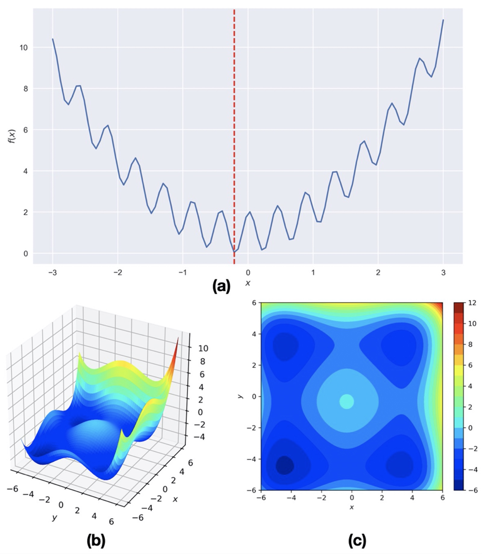
Global vs. Local Optimization
Consider a hypothetical multi-modal function:
Genetic Algorithm
Genetic algorithm (GA), first proposed by John Holland in 1975 and described in Goldberg (1988), is based on analogies with biological evolution processes. The principle of GA is quite simple and mirrors what is perceived to occur in evolutionary mechanisms. The idea is to start with a given set of feasible trial solutions (either constrained or unconstrained) and iteratively evaluate objective (or fitness) function by keeping only those solutions that give the optimal value of the objective function and randomly mutate them to try and do even better and successive iterations. Thus, the beneficial mutations (that lead to optimal values) are kept while those that perform poorly are thrown away, i.e., the survival of the fittest.
Key idea — evolution as a search strategy. A GA does not follow a gradient toward the answer; instead it keeps a whole population of candidate solutions and lets them compete. Each generation, the fittest survive (low objective value), swap pieces of their “genes” via crossover, and get random tweaks via mutation. Because many candidates explore the space at once — and mutation keeps injecting fresh guesses — a GA can climb out of local minima where a gradient method would get stuck. The price is many objective-function evaluations and a stochastic answer, so you run it several times and average.
Consider the unconstrained optimization problem with the objective function $\min f(\vec{x})$ where $\vec{x}$ is an $n$-dimensional vector. Suppose $m$ initial guesses are given for the values of $\vec{x}$ so that
\[\textrm{guess } j \textrm{ is } x_j\]Thus $m$ solutions are evaluated and compared with each other in order to see which of the solutions generate the smallest objective function since our goal (in general) is to minimize it. We can order the guesses such that the first $p < m$ give the smallest values of $f(\vec{x})$. Arranging our data, we have
\[\begin{aligned} & \textrm{keep } x_j, \quad j = 1, 2, \ldots, p \\ & \textrm{discard } x_j, \quad j = p+1, p+2, \ldots, m \end{aligned}\]Since the first $p$ solutions are the best, these are kept in the next generation. In addition, we now generate $m-p$ new trial solutions that are randomly mutated from the $p$ best solutions. This process is repeated through a finite number of iterations with the hope that convergence to the optimal solution is achieved.
Scheme
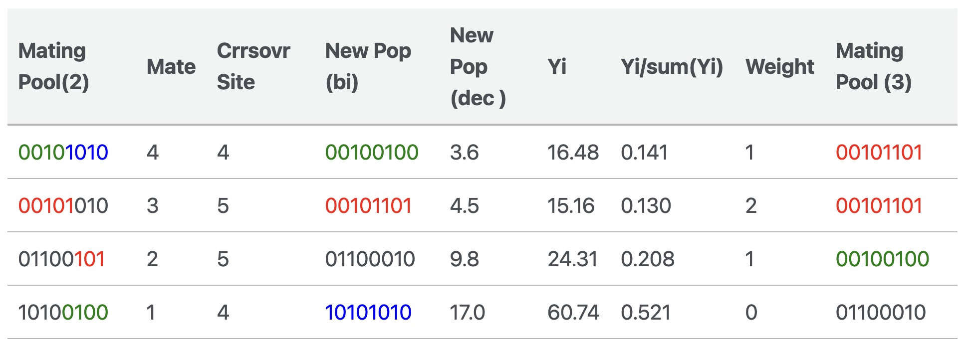
The steps involved in the Genetic Algorithm are:
- The initial population of model parameters is randomly chosen within the given search range.
- The simple GA undergoes a set of operations on the model population to produce the next generation: selection, coding, crossover, and mutation.
- In the selection scheme, the model parameters exhibiting the higher fitness value (lower objective function value relative to others) are selected and replicated with the given probability. The total population size remains constant; then, the population members are randomly paired among themselves.
- In the coding scheme, each population’s decimal values are converted to a binary system, forming a long bit string (analogous to a chromosome).
- In the crossover scheme, some part of the long bit string of binary model parameters is exchanged with their corresponding pair to produce a new population.
- In the mutation scheme, some randomly selected sites (with a given probability) of the new set of the binary model population are switched.
- These sets of operations will continue until some pre-defined termination criteria for the technique are satisfied.
The Optimum size of a coffee mug for a Café owner?
Here, the objective function is to minimize the loss of the Café owner. Let us make a very simple function for that.
\[y = 0.2 x^2 + 50/x\]where $x$ is the size of the coffee mug. If the coffee mug’s size is too small, then the customers may not like it, and if the size is too large, then the owner will have to endure loss, hence the hypothetical function. We assumed that the price of the coffee is fixed.
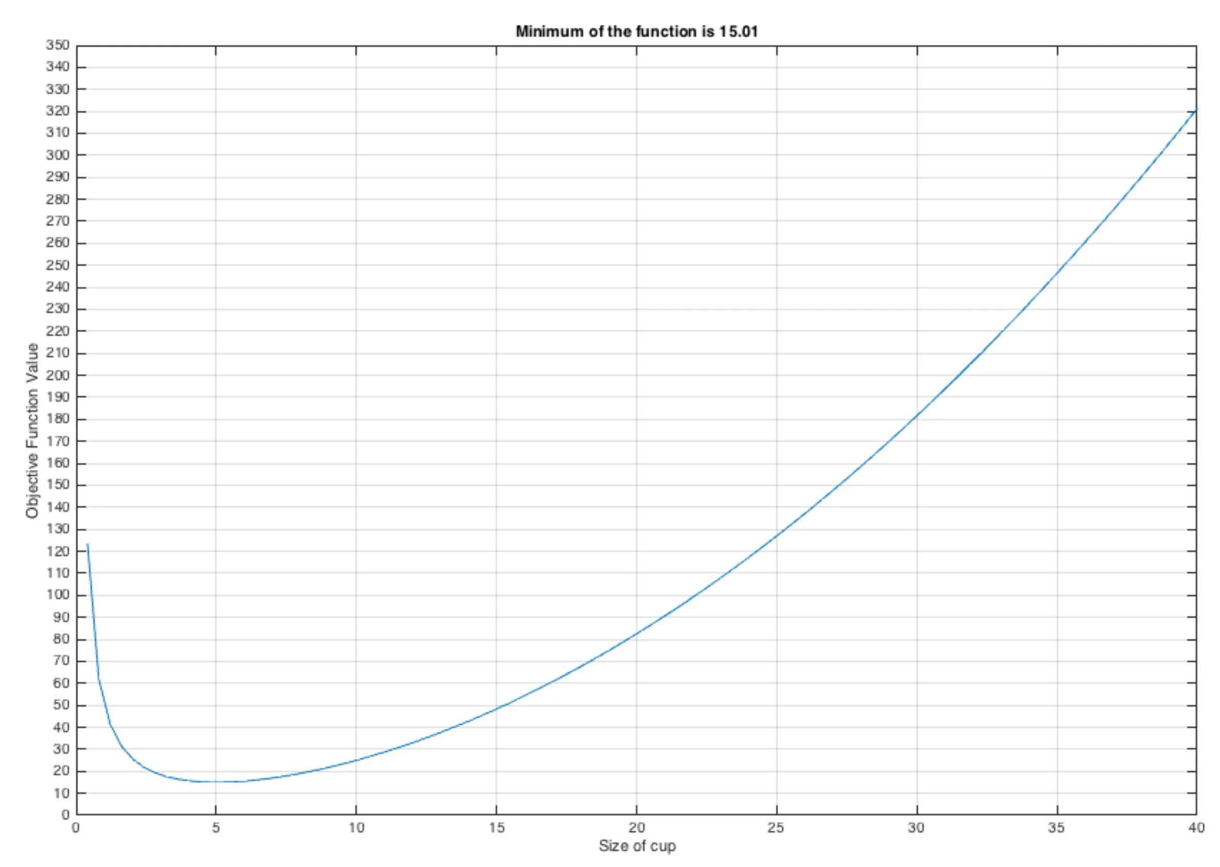
Solution
Let us solve this iteratively:
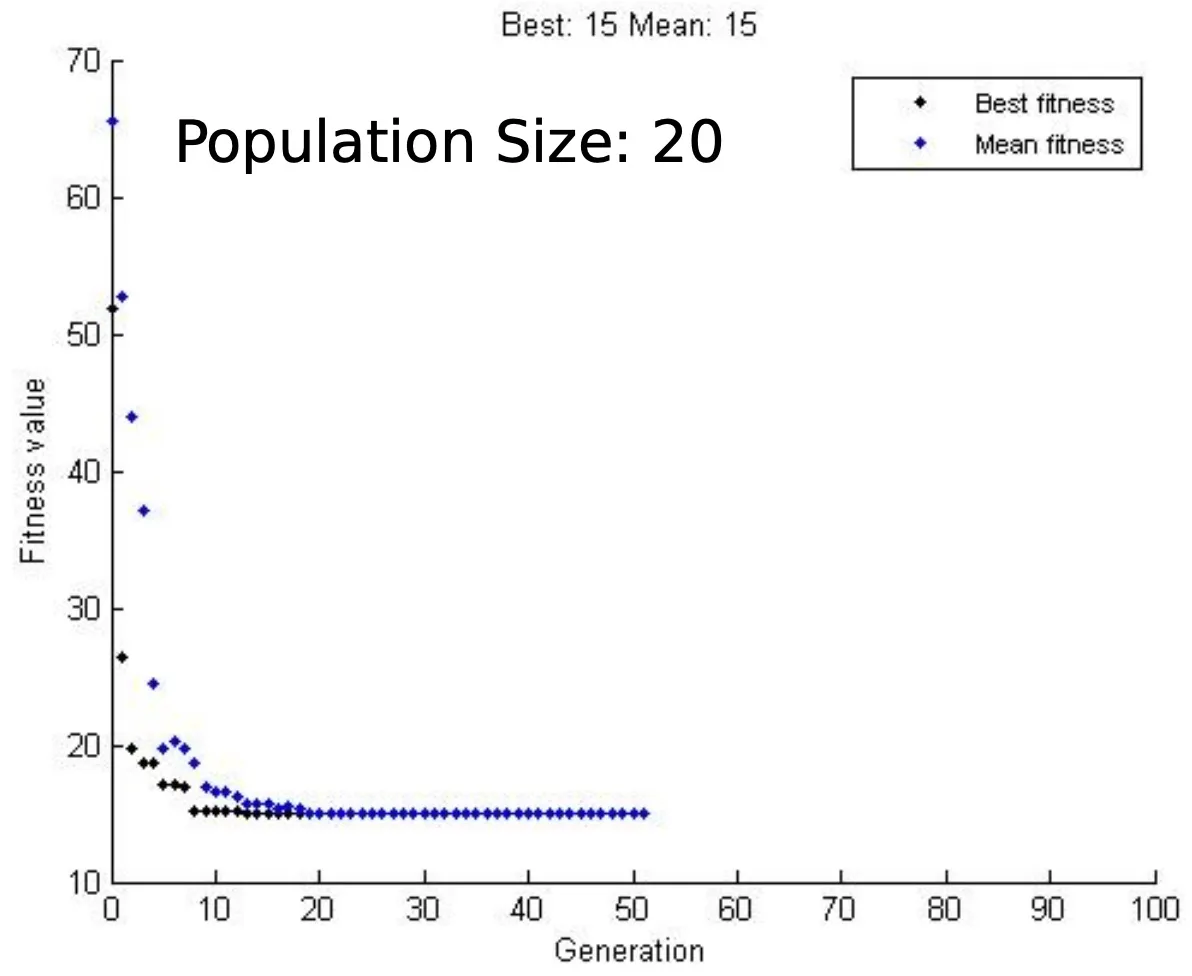
Generation 1
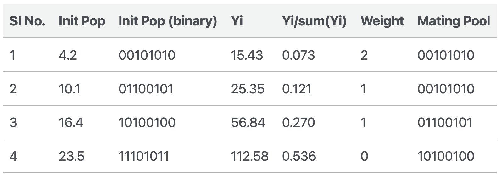
The average fitness in this generation is : 52.55.
Generation 2
The average fitness in this generation is 29.17. We can continue iterating as long as our termination criteria are satisfied. Some of the standard termination criteria are the tolerance value (the difference in the fitness of the generation compared to the previous generation), the maximum number of generations, etc.
Fitness with generations
Earthquake location using Genetic Algorithm
In this series of earthquake location problems, we have used the Monte Carlo method for the earthquake location that gives us reliable results. The earthquake location problem was introduced in the previous post.
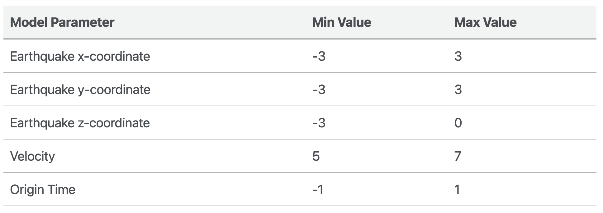
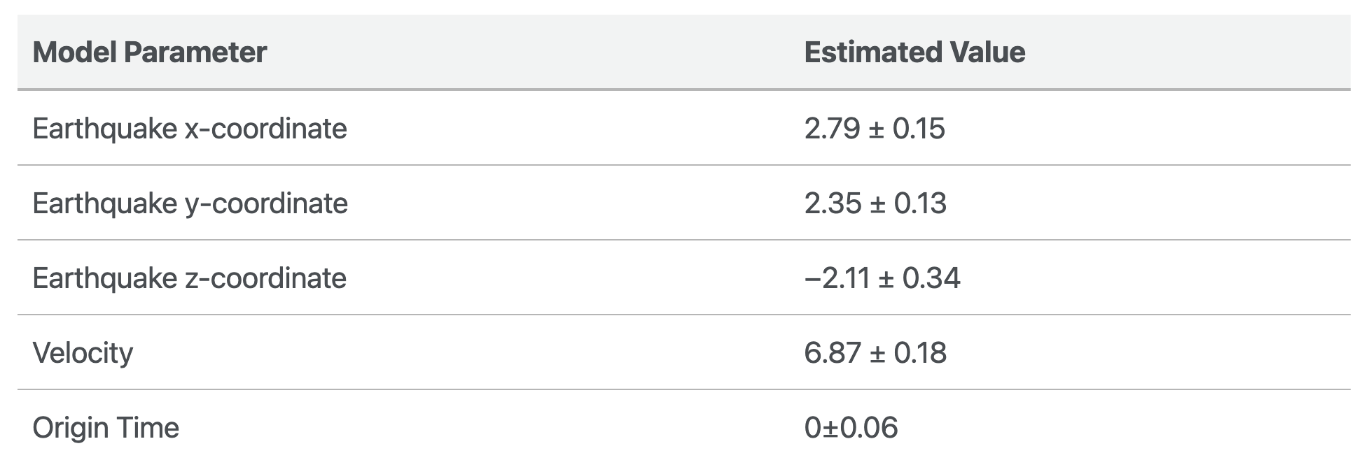
Now, I applied GA from the direct search toolbox of MATLAB to find the solution of the best earthquake location parameters for the earthquake problem defined in previous post for 30 stations. The GA does not improve the solutions but similar to the Monte Carlo method; it allows a large model space to be searched for solutions. I used the lower and upper limits for the search of best parameters as defined in Table 1. After 85 generations of a run and terminated based on the tolerance criterion, the best parameters found by the GA are [2.9750 2.5202 -2.5535 6.6696 -0.0839]. Since GA is a stochastic optimization scheme, it is best practice to make a reasonable number of acceptable solutions and consider its mean as the final solution. For the 50 runs of the GA for the earthquake location problem, the estimated mean and std of the model parameters are shown in Table 2. The difference from the actual model parameters arises because of random noise in the observed arrival time data.
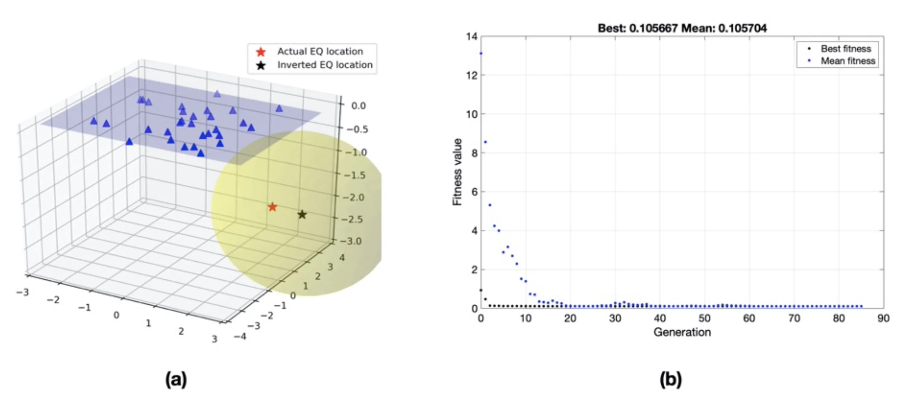
(a) Estimated location of a hypothetical earthquake using Genetic algorithm. The yellow ellipsoid shows the 1𝜎 confidence interval in the hypocenter location. (b) Fitness value versus generations. The best score value (0.106) and mean score (0.106) versus generation for estimating earthquake location parameters using genetic algorithm scheme.
lower=[-3 -3 -3 5 -1];
upper=[3 3 0 7 1];
options = optimoptions('ga','PlotFcn', @gaplotbestf,'Display','iter'); 6. x=ga(@(pp)fit_arrival_times(pp),5,[],[],[],[],lower,upper,[],options)

function E=fit_arrival_times(pp)
filename = 'arrival_times.csv';
[dobs, dpre] = read_arrivaltimes(filename);

stationlocations = read_stnloc('station_locations.csv', 2, 31);
d_pre = zeros(length(stationlocations),1);

for i=1:length(stationlocations)
    dist = sqrt((pp(1) - stationlocations(i,1))^2 + (pp(2) - stationlocations( i,2))^2 + (pp(3) - stationlocations(i,3))^2);
    arr = dist/pp(4) + pp(5);
    d_pre(i) = arr;
end
E=sum((dobs-d_pre).^2);
No MATLAB? Use a Python equivalent. The ga solver above comes from MATLAB’s Global Optimization Toolbox and is still current. If you would rather stay in Python, scipy.optimize.differential_evolution is a batteries-included, gradient-free global optimizer in SciPy that fits the same “minimize an objective over bounds” pattern — you pass your fit_arrival_times-style cost function and the [lower, upper] bounds. For a dedicated GA library, PyGAD and DEAP expose the selection/crossover/mutation operators directly.
Complete codes
Complete codes can be downloaded from my github repository
Quick check: Which feature of a genetic algorithm most helps it avoid getting trapped in a local minimum of a multi-modal objective function?
- It follows the steepest downhill gradient at every step
- It keeps a whole population and injects randomness via mutation, exploring many regions at once
- It always converges in a fixed number of iterations
- It requires the objective function to be differentiable
Recap
- Optimization picks the best model under some criterion; geophysical objective functions are often multi-modal, so a purely downhill (local) method can settle into the wrong minimum.
- A genetic algorithm evolves a population of candidate solutions through selection → crossover → mutation, generation after generation, until a termination criterion (tolerance or max generations) is met.
- Because many candidates search in parallel and mutation keeps adding randomness, a GA explores a large model space and is robust to local minima — at the cost of many function evaluations.
- GA is stochastic: run it several times and report the mean (and spread) of the solutions, as done here over 50 runs of the earthquake-location problem.
- In practice you rarely code the operators by hand — MATLAB’s
ga, SciPy’sdifferential_evolution, or PyGAD/DEAP handle the mechanics for you.
Where to go next
- Solving a toy earthquake-location problem using a genetic algorithm — a hands-on, from-scratch GA walkthrough in Python.
- An introduction to the genetic algorithm (geophysics companion post) — the same method with worked binary crossover/mutation tables.
- The earthquake location problem and the least-squares method — the local-inversion baseline this post improves on.
- Monte Carlo methods and the earthquake location problem — another global, sampling-based search over the same model space.
Disclaimer of liability
The information provided by the Earth Inversion is made available for educational purposes only.
Whilst we endeavor to keep the information up-to-date and correct. Earth Inversion makes no representations or warranties of any kind, express or implied about the completeness, accuracy, reliability, suitability or availability with respect to the website or the information, products, services or related graphics content on the website for any purpose.
UNDER NO CIRCUMSTANCE SHALL WE HAVE ANY LIABILITY TO YOU FOR ANY LOSS OR DAMAGE OF ANY KIND INCURRED AS A RESULT OF THE USE OF THE SITE OR RELIANCE ON ANY INFORMATION PROVIDED ON THE SITE. ANY RELIANCE YOU PLACED ON SUCH MATERIAL IS THEREFORE STRICTLY AT YOUR OWN RISK.
Leave a comment