Solving a Toy Earthquake Location Problem Using a Genetic Algorithm

Utpal Kumar 13 minute read DATASCIENCE September 07, 2024

Introduction

Locating an earthquake from seismic data is a classic inverse problem: from the observed arrival times of seismic waves at several stations, estimate the event’s origin coordinates, depth, and time. Traditional methods often lean on linearization and a good initial guess. A Genetic Algorithm (GA) takes a different route — it evolves a population of candidate locations toward the best fit, no derivatives required.

In this article I walk through the earthquake location problem and solve it with a GA. If you’re new to Genetic Algorithms, start here first: Genetic Algorithm: a highly robust inversion scheme for geophysical applications.

The one mental model

Treat the earthquake location as a search problem over five unknowns — position $(x, y, z)$, velocity $v$, and origin time $t_0$. For any guess you can predict the arrival times and compare them to what was observed; the mismatch is the fitness. The GA breeds better guesses generation after generation until the mismatch is as small as it can make it.

The problem, formalized

For a candidate source at $(x, y, z)$ with velocity $v$ and origin time $t_0$, the predicted arrival time at station $i$ located at $(x_i, y_i, z_i)$ is just distance over speed plus the origin time:

\[t_i^{\mathrm{pred}} = \frac{\sqrt{(x-x_i)^2 + (y-y_i)^2 + (z-z_i)^2}}{v} + t_0\]

The GA searches for the parameters that make those predictions match the observations. The fitness (which we minimize) is the sum of squared residuals across all $N$ stations:

\[E(x, y, z, v, t_0) = \sum_{i=1}^{N} \left( t_i^{\mathrm{obs}} - t_i^{\mathrm{pred}} \right)^2\]

That’s exactly what fitness_function computes in the code below, and calc_arrival_time implements the first equation.

Check your understanding

What is the GA actually minimizing?

How the genetic algorithm works

Each generation repeats the same four steps — the population gets a little fitter each time around:

After 200 generations, the fittest individual ever seen (kept in the hall of fame) is the estimated location.

Complete script

import os
import numpy as np
import pandas as pd
import numpy.linalg as linalg
from deap import base, creator, tools, algorithms
from mayavi import mlab
import noise
import matplotlib.pyplot as plt

np.random.seed(0)

# Define the boundaries of the grid to be used in simulations
minx, maxx = -5, 5
miny, maxy = -5, 5

# Set constraints on depth, reflecting realistic limits
depth_min = -3
depth_max = 0

# Create a directory to save intermediate steps of the genetic algorithm
output_dir = "ga_steps"
os.makedirs(output_dir, exist_ok=True)


# Part 1: Generate synthetic data representing an earthquake and seismic stations
def generate_data():
    error = 0.05  # Introduce a 5% error in the initial guess
    numstations = 30  # Define the number of seismic stations

    # Randomly place seismic stations within the defined grid boundaries
    stn_locs = []
    xvals = minx + (maxx - minx) * np.random.rand(numstations)
    yvals = miny + (maxy - miny) * np.random.rand(numstations)
    for num in range(numstations):
        stn_locs.append([xvals[num], yvals[num], 0])

    # Define the actual earthquake location
    eq_loc = [2, 2, -2]  # Coordinates in km
    vel = 6  # Velocity in km/s
    origintime = 0  # Origin time of the earthquake

    # Function to calculate arrival times of seismic waves at the stations
    def calc_arrival_time(eq_loc, stnx, stny, stnz, vel, origintime):
        eqx, eqy, eqz = eq_loc
        dist = np.sqrt((eqx - stnx) ** 2 + (eqy - stny) ** 2 + (eqz - stnz) ** 2)
        arr = dist / vel + origintime
        return arr

    # Generate an initial guess of the earthquake location with some error
    eq_initial_guess = [
        eq_loc[0] + error * eq_loc[0],
        eq_loc[1] + error * eq_loc[1],
        eq_loc[2] + error * eq_loc[2],
    ]
    m_intial = [
        eq_initial_guess[0],
        eq_initial_guess[1],
        eq_initial_guess[2],
        vel + error * vel,
        origintime + error * origintime,
    ]

    d_obs = []  # Observed arrival times
    d_pre = []  # Predicted arrival times based on the initial guess
    noise_level_data = 0.05  # Introduce a 5% noise level

    # Calculate observed and predicted arrival times at each station
    for stnx, stny, stnz in stn_locs:
        arr = calc_arrival_time(eq_loc, stnx, stny, stnz, vel, origintime)
        noise_val = np.random.normal(loc=0, scale=noise_level_data * arr)
        d_obs.append(arr + noise_val)
        d_pre.append(calc_arrival_time(eq_initial_guess, stnx, stny, stnz, m_intial[3], m_intial[4]))

    # Save the observed and predicted data to CSV files
    arr_df = pd.DataFrame({"dobs": d_obs, "d_pre": d_pre})
    arr_df.to_csv("arrival_times.csv", index=False)

    stn_locs = np.array(stn_locs)
    station_loc_df = pd.DataFrame({"xloc": stn_locs[:, 0], "yloc": stn_locs[:, 1], "zloc": stn_locs[:, 2]})
    station_loc_df.to_csv("station_locations.csv", index=False)

    return eq_loc, stn_locs, noise_level_data


# Part 2: Implement the Genetic Algorithm (GA) for earthquake location estimation
def read_arrivaltimes(filename):
    data = np.loadtxt(filename, delimiter=",", skiprows=1)
    dobs = data[:, 0]
    return dobs


def read_stnloc(filename):
    station_locations = np.loadtxt(filename, delimiter=",", skiprows=1)
    return station_locations


def fitness_function(params):
    # Apply depth constraints to the parameters
    if params[2] < depth_min or params[2] > depth_max:
        return float("inf"),  # Penalize solutions that violate the depth constraint

    station_locations = read_stnloc("station_locations.csv")
    observed_arrival_times = read_arrivaltimes("arrival_times.csv")

    # Extract parameters from the individual
    x, y, z, velocity, origin_time = params
    predicted_arrival_times = []

    # Calculate predicted arrival times based on the current guess
    for station in station_locations:
        dist = np.sqrt((x - station[0]) ** 2 + (y - station[1]) ** 2 + (z - station[2]) ** 2)
        arrival_time = dist / velocity + origin_time
        predicted_arrival_times.append(arrival_time)

    # Calculate the error between observed and predicted arrival times
    predicted_arrival_times = np.array(predicted_arrival_times)
    error = np.sum((observed_arrival_times - predicted_arrival_times) ** 2)
    return error,


# Run the genetic algorithm to optimize earthquake location
def run_ga(visualize_steps=False):
    # Define a minimization problem with fitness based on minimizing the error
    if "FitnessMin" not in creator.__dict__:
        creator.create("FitnessMin", base.Fitness, weights=(-1.0,))
    if "Individual" not in creator.__dict__:
        creator.create("Individual", list, fitness=creator.FitnessMin)

    # Set up the genetic algorithm toolbox
    toolbox = base.Toolbox()
    toolbox.register("attr_float", np.random.uniform, -3, 3)
    toolbox.register("individual", tools.initRepeat, creator.Individual, toolbox.attr_float, n=5)
    toolbox.register("population", tools.initRepeat, list, toolbox.individual)
    toolbox.register("mate", tools.cxBlend, alpha=0.5)
    toolbox.register("mutate", tools.mutGaussian, mu=0, sigma=1, indpb=0.2)
    toolbox.register("select", tools.selTournament, tournsize=3)
    toolbox.register("evaluate", fitness_function)

    # Initialize the population and parameters for the genetic algorithm
    population = toolbox.population(n=300)
    n_generations = 200
    cxpb = 0.7  # Crossover probability
    mutpb = 0.3  # Mutation probability

    # Track the best individual and statistics during the run
    hall_of_fame = tools.HallOfFame(1)
    stats = tools.Statistics(lambda ind: ind.fitness.values)
    stats.register("min", np.min)
    stats.register("mean", np.mean)
    logbook = tools.Logbook()
    logbook.header = ["gen", "min", "mean"]

    # Main loop to run the genetic algorithm
    for gen in range(n_generations):
        population, _ = algorithms.eaSimple(population, toolbox, cxpb=cxpb, mutpb=mutpb, ngen=1, verbose=False)

        # Apply depth constraints after mutation
        for ind in population:
            if ind[2] < depth_min:
                ind[2] = depth_min
            elif ind[2] > depth_max:
                ind[2] = depth_max

        # Record statistics and update the hall of fame
        record = stats.compile(population)
        logbook.record(gen=gen, **record)
        hall_of_fame.update(population)

        # Optionally visualize intermediate steps
        if visualize_steps and gen % 10 == 0:
            save_intermediate_plot(population, hall_of_fame, gen)

    # Return the best solution found by the algorithm
    best_individual = hall_of_fame[0]
    best_fitness = fitness_function(best_individual)[0]

    return best_individual, best_fitness, logbook


# Placeholder for intermediate plot saving, if needed for debugging or analysis
def save_intermediate_plot(population, hall_of_fame, gen):
    pass


# Part 3: Estimate an ellipsoid around the best estimated earthquake location
def estimate_ellipsoid(center, location_error, noise_level):
    # Combine location error and noise level to form the ellipsoid's radii
    coeffs = location_error + noise_level
    A = np.array([[coeffs[0], 0, 0], [0, coeffs[1], 0], [0, 0, coeffs[2]]])
    _, s, rotation = linalg.svd(A)

    # Handle potential division by zero
    s = np.where(s == 0, 1e-10, s)
    radii = 1.0 / np.sqrt(s)

    u = np.linspace(0.0, 2.0 * np.pi, 100)
    v = np.linspace(0.0, np.pi, 100)

    xx = radii[0] * np.outer(np.cos(u), np.sin(v))
    yy = radii[1] * np.outer(np.sin(u), np.sin(v))
    zz = radii[2] * np.outer(np.ones_like(u), np.cos(v))

    # Rotate and translate the ellipsoid to the estimated location
    for i in range(len(u)):
        for j in range(len(v)):
            [xx[i, j], yy[i, j], zz[i, j]] = np.dot([xx[i, j], yy[i, j], zz[i, j]], rotation) + center

    return xx, yy, zz


# Part 4: Visualization of results with Mayavi, including rough topography
def generate_rough_topography(X, Y, scale=1.0, octaves=6, persistence=0.5, lacunarity=2.0):
    # Generate a rough topography using Perlin noise
    Z = np.zeros_like(X)
    for i in range(X.shape[0]):
        for j in range(X.shape[1]):
            Z[i, j] = noise.pnoise2(X[i, j] * scale, Y[i, j] * scale, octaves=octaves,
                                    persistence=persistence, lacunarity=lacunarity)
    return Z


def plot_results_with_mayavi(eq_loc, stn_locs, best_params, noise_level):
    location_error = np.abs(np.array(eq_loc) - np.array(best_params[:3]))

    # Initialize the Mayavi figure
    mlab.figure(size=(1000, 800), bgcolor=(0.2, 0.2, 0.2))

    # Generate and plot the rough topography surface
    X, Y = np.mgrid[minx:maxx:200j, miny:maxy:200j]
    Z = generate_rough_topography(X, Y, scale=0.5)
    mlab.surf(X, Y, Z, colormap="terrain", warp_scale=1.0)

    # Plot station locations
    mlab.points3d(stn_locs[:, 0], stn_locs[:, 1], stn_locs[:, 2],
                  color=(0.1, 0.5, 1), scale_factor=0.3, mode="cube", opacity=1)

    # Actual earthquake location in red
    mlab.points3d(eq_loc[0], eq_loc[1], eq_loc[2], color=(1, 0.3, 0.3), scale_factor=0.6, mode="sphere")

    # Estimated location in green
    mlab.points3d(best_params[0], best_params[1], best_params[2],
                  color=(0.3, 1, 0.3), scale_factor=0.6, mode="sphere")

    # Error ellipsoid around estimated location
    if np.any(location_error + noise_level > 0):
        center = [best_params[0], best_params[1], best_params[2]]
        xx, yy, zz = estimate_ellipsoid(center, location_error, [noise_level] * 3)
        ellipsoid = mlab.mesh(xx, yy, zz, color=(1, 1, 0.6), opacity=0.6)
        ellipsoid.actor.property.interpolation = "phong"
        ellipsoid.actor.property.specular = 0.1
        ellipsoid.actor.property.specular_power = 20
        ellipsoid.actor.property.diffuse = 0.5
        ellipsoid.actor.property.ambient = 0.3

    # Camera view and axes
    mlab.view(azimuth=45, elevation=75, distance=30)
    mlab.axes(color=(1, 1, 1), xlabel="X (km)", ylabel="Y (km)", zlabel="Depth (km)")
    mlab.outline(color=(1, 1, 1))

    mlab.savefig("earthquake_loc_ga_mayavi.png", magnification=3)
    mlab.clf()


# Alternative visualization with Matplotlib
def plot_results(eq_loc, stn_locs, best_params, noise_level):
    location_error = np.abs(np.array(eq_loc) - np.array(best_params[:3]))

    fig = plt.figure()
    ax = plt.axes(projection="3d")

    X, Y = np.mgrid[minx:maxx:200j, miny:maxy:200j]
    Z = generate_rough_topography(X, Y, scale=0.5)
    ax.plot_surface(X, Y, Z, rstride=1, cstride=1, cmap="terrain", edgecolor="none", alpha=0.7)

    elevated_z = np.array([x[2] + 0.05 for x in stn_locs])
    ax.scatter([x[0] for x in stn_locs], [x[1] for x in stn_locs], elevated_z,
               c="blue", marker="s", s=120, label="Stations", edgecolors="k")

    ax.scatter(eq_loc[0], eq_loc[1], eq_loc[2], c="red", marker="o", s=100,
               label=f"Actual EQ location ({eq_loc[0]:.2f}, {eq_loc[1]:.2f}, {eq_loc[2]:.2f})")

    ax.scatter(best_params[0], best_params[1], best_params[2], c="green", marker="*", s=150,
               label=f"Estimated EQ location ({best_params[0]:.2f}, {best_params[1]:.2f}, {best_params[2]:.2f})")

    if np.any(location_error + noise_level > 0):
        center = [best_params[0], best_params[1], best_params[2]]
        xx, yy, zz = estimate_ellipsoid(center, location_error, [noise_level] * 3)
        ax.plot_surface(xx, yy, zz, rstride=4, cstride=4, color="yellow", alpha=0.3, edgecolor="none")

    ax.set_xlim([minx, maxx])
    ax.set_ylim([miny, maxy])
    ax.set_zlim([-5, 0.1])
    ax.set_xlabel("X Coordinate")
    ax.set_ylabel("Y Coordinate")
    ax.set_zlabel("Depth")
    ax.view_init(elev=30, azim=60)

    ax.legend(loc="lower left")
    plt.tight_layout()
    plt.savefig("earthquake_loc_ga.png", bbox_inches="tight", dpi=300)


# Main execution block
if __name__ == "__main__":
    eq_loc, stn_locs, noise_level = generate_data()
    best_params, best_fitness, _ = run_ga(visualize_steps=True)

    plot_results_with_mayavi(eq_loc, stn_locs, best_params, noise_level)
    plot_results(eq_loc, stn_locs, best_params, noise_level)

    print(f"Actual EQ Location: {eq_loc}")
    print(f"Best Estimated EQ Location: {best_params}")
    print(f"Location Error: {np.abs(np.array(eq_loc) - np.array(best_params[:3]))}")
    print(f"Best Fitness (Error): {best_fitness}")

Here is a brief explanation of the code used in the process:

Data Generation: The function generate_data() simulates an earthquake event and the corresponding seismic station observations. It introduces errors and noise to mimic real-world data.
Genetic Algorithm: The run_ga() function executes the Genetic Algorithm, using a fitness function (fitness_function()) to evaluate how close each candidate solution is to the actual earthquake location.
Visualization: plot_results_with_mayavi() and plot_results() create visual representations of the results. Mayavi is used for more detailed 3D plots, while Matplotlib provides an alternative.
Error Analysis: The code calculates and visualizes the error between the actual and estimated earthquake locations, providing a clear measure of the GA’s effectiveness.

Generating synthetic seismic data

To tackle the earthquake location problem, we first need to generate synthetic data that mimics real seismic observations. This involves placing seismic stations randomly within a defined grid and simulating the arrival times of seismic waves at these stations based on a known earthquake location.

Here is a breakdown of the process:

Grid Boundaries: The simulation grid is defined with x and y boundaries ranging from -5 to 5 km. The depth is constrained between -3 and 0 km to reflect realistic limits.
Station Placement: 30 seismic stations are randomly distributed within the grid.
True Earthquake Location: The actual earthquake is set at coordinates (2, 2, -2) km.
Arrival Times: The arrival times of seismic waves at each station are calculated using the distance from the earthquake location and the wave velocity. To simulate real-world conditions, we introduce a small amount of noise into these times.

The synthetic data generated serves as the basis for our Genetic Algorithm to estimate the earthquake’s location.

Implementing the genetic algorithm

The core of this approach is a Genetic Algorithm that iteratively searches for the best solution to the earthquake location problem. The GA starts with a population of random solutions and evolves them over generations using operations inspired by natural selection: crossover, mutation, and selection.

Here is a step-by-step explanation:

Fitness Function: The fitness function measures how well a candidate solution predicts the observed arrival times. It calculates the error between the observed and predicted times. The goal is to minimize this error.
Population Initialization: The algorithm begins with a population of 300 random individuals, each representing a potential earthquake location and other parameters (velocity and origin time).
Evolution Process: Over 200 generations, the population evolves through crossover (combining two solutions) and mutation (randomly altering a solution) to produce new solutions. The best solutions are selected to continue to the next generation.
Depth Constraints: To ensure realistic results, we apply constraints on the depth of the earthquake during the mutation step.

The GA runs until it finds the best solution, i.e., the set of parameters that minimize the error in predicting the observed arrival times.

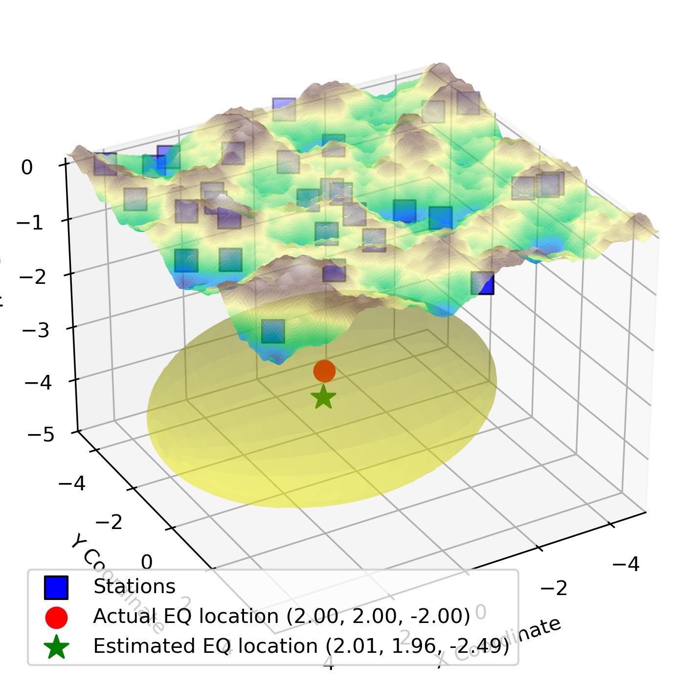
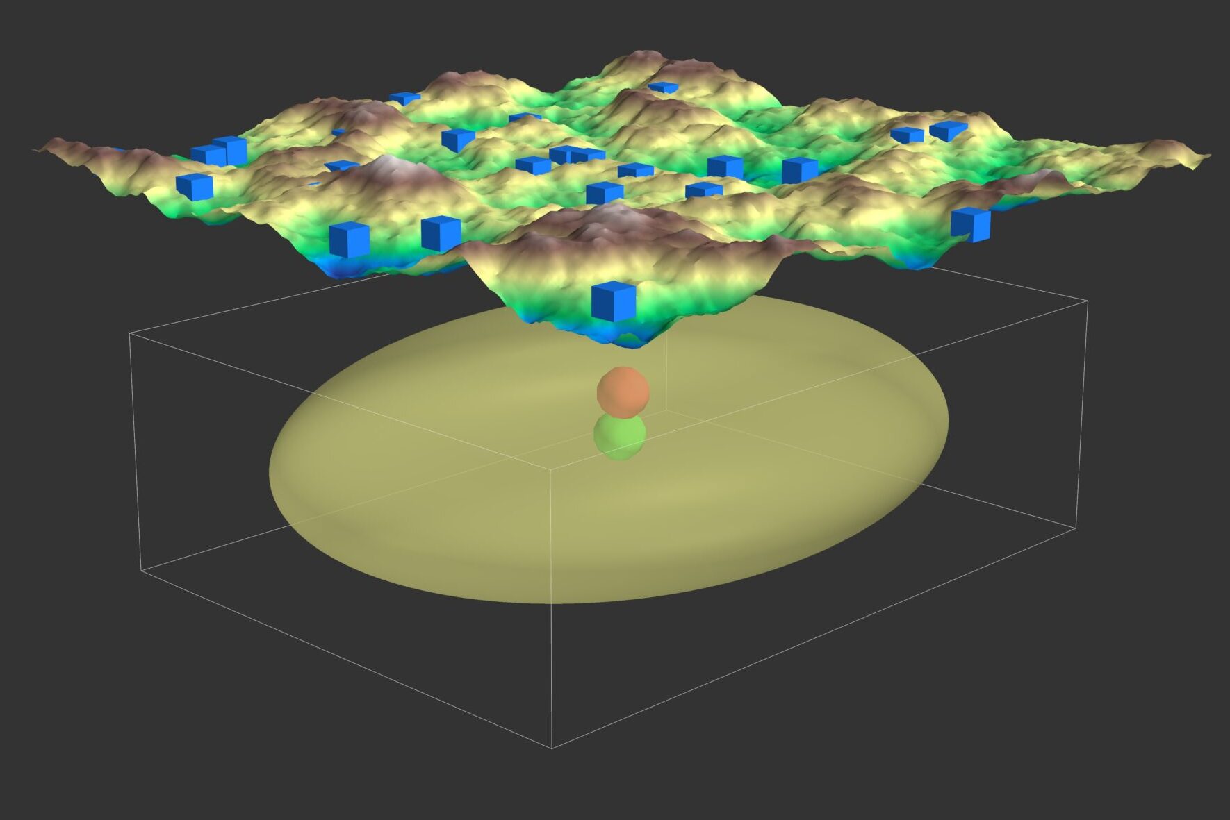
Visualizing the results

Once the Genetic Algorithm identifies the best solution, we visualize the estimated earthquake location and compare it to the actual location. The visualization includes:

Station Locations: Displayed as blue cubes on a 3D plot.
Actual and Estimated Locations: Highlighted as red and green spheres, respectively.
Error Ellipsoid: An ellipsoid around the estimated location representing the uncertainty in the solution.

We use Mayavi for interactive 3D visualization and Matplotlib for static 3D plots. These visualizations provide insights into the accuracy of the GA in solving the earthquake location problem.

Earthquake Location using Genetic Algorithm (MATPLOTLIB)

Earthquake Location using Genetic Algorithm (MAYAVI)

Video Walkthrough

The fine print: 8 limitations of this toy example

While the GA is a robust approach, this demonstration makes simplifying assumptions worth keeping in mind:

Simplified grid and depth constraints: the grid spans only −5 to 5 km with depth confined to −3 to 0 km. Real problems cover much larger areas and more complex depth variation.
Synthetic data with simplified assumptions: a constant velocity (6 km/s) and known origin time. Real subsurface velocities are heterogeneous, and origin time is usually uncertain.
Noise and error representation: a fixed 5% noise level. Real seismic noise is more complex and variable (instruments, environment, human activity).
Limited number of stations: 30 stations. Real networks have more stations over larger areas, improving accuracy.
Fitness-function simplification: it assumes arrival-time misfit is the only error source. Velocity-model or station-location errors complicate the fitness landscape.
Algorithm parameters and convergence: population size, mutation, and crossover are standard defaults; the GA can converge to a local rather than global minimum.
Visualization and interpretation: the error ellipsoid is an approximation of uncertainty and depends on the underlying assumptions.
Scalability to real-world applications: large-scale problems need more stations, data, and compute — often parallel processing and more sophisticated fitness functions.

Recap

Without scrolling up — can you frame the method? Solving the earthquake location problem with a GA means:

Treat it as a search over $(x, y, z, v, t_0)$,
Score each guess by the squared misfit $E = \sum (t^{\mathrm{obs}} - t^{\mathrm{pred}})^2$,
Evolve a population — initialize → evaluate → select → crossover + mutate — for 200 generations,
Take the fittest individual as the estimate, with an error ellipsoid for uncertainty.

The GA needs no derivatives and no linearization, which is exactly what makes it a friendly entry point to inversion — at the cost of the assumptions listed above.

Conclusion

The Genetic Algorithm offers a powerful, derivative-free method for the earthquake location problem, handling noise and uncertainty gracefully. For more on Genetic Algorithms and their applications, see my earlier post: Genetic Algorithm: a highly robust inversion scheme for geophysical applications.

Disclaimer of liability

The information provided by the Earth Inversion is made available for educational purposes only.

Whilst we endeavor to keep the information up-to-date and correct. Earth Inversion makes no representations or warranties of any kind, express or implied about the completeness, accuracy, reliability, suitability or availability with respect to the website or the information, products, services or related graphics content on the website for any purpose.

UNDER NO CIRCUMSTANCE SHALL WE HAVE ANY LIABILITY TO YOU FOR ANY LOSS OR DAMAGE OF ANY KIND INCURRED AS A RESULT OF THE USE OF THE SITE OR RELIANCE ON ANY INFORMATION PROVIDED ON THE SITE. ANY RELIANCE YOU PLACED ON SUCH MATERIAL IS THEREFORE STRICTLY AT YOUR OWN RISK.