Markov Chain Monte Carlo for Geoscientists
Imagine being handed the strangest field assignment in geophysics. You are dropped into a landscape covered in fog so thick you can never see more than one step ahead. You carry a single instrument — an altimeter that reads relative height only — and your job is to produce a map of where the terrain is high. You cannot survey the whole landscape. All you can do is walk, one step at a time, following a simple rule. And yet, given enough steps, the density of your footprints becomes a faithful map of the high ground.
That is Markov Chain Monte Carlo (MCMC). The name describes exactly what it is: a Markov chain because each step depends only on the current position (no memory, no map), and Monte Carlo because the steps are random. The rest of this post unpacks the walking rule, shows it working on a problem where we know the exact answer, and then puts it to work on a real geophysical task: locating an earthquake from arrival times.
The one idea
MCMC turns a question we cannot answer directly — what does the whole posterior distribution look like? — into one we can: where does a walker following a simple accept/reject rule spend its time? Time spent at a location is proportional to probability. The histogram of the walker’s positions is the posterior.
Why a geoscientist should care
Nearly every quantitative problem in geoscience is an inverse problem: we observe data at the surface (arrival times, gravity, radiocarbon dates, waveforms) and want the model parameters that produced them (a hypocenter, a density structure, an age–depth curve, a velocity model). And as I discussed in the NonLinLoc post, the honest answer to an inverse problem is not a point — it is a probability distribution over all the models consistent with the data.
NonLinLoc can afford to map that distribution exhaustively because a hypocenter has only 3–4 unknowns: a grid of 100 nodes per axis costs $100^3 = 10^6$ evaluations. Cheap. But suppose your model has 20 parameters — a modest layered velocity model, say. The same grid now costs $100^{20} = 10^{40}$ evaluations. At a million evaluations per second that is about $3\times10^{26}$ years. The universe is about $1.4\times10^{10}$ years old. This explosion is the curse of dimensionality, and it kills every “just evaluate everywhere” strategy — grids, and also the naive uniform random sampling I used in my earlier post on Monte Carlo methods and earthquake location, which wastes almost every sample on regions of negligible probability.
What we need is a sampler that spends its effort where the probability actually is. That is exactly what the foggy walk does.
Bayes in one breath
Write the model parameters as $\mathbf{m}$ and the observed data as $\mathbf{d}$. Bayes’ rule says:
\[\underbrace{p(\mathbf{m}\mid \mathbf{d})}_{\text{posterior}} \;\propto\; \underbrace{p(\mathbf{d}\mid \mathbf{m})}_{\text{likelihood (data fit)}} \;\cdot\; \underbrace{p(\mathbf{m})}_{\text{prior}}\]The posterior $p(\mathbf{m}\mid\mathbf{d})$ is the “terrain” our walker explores: for every candidate model it gives a height — how plausible that model is, given the data and what we knew beforehand. High ground = models that fit well; fog = we can only evaluate the height where we stand, never see the whole surface at once.
Notice the $\propto$ sign. The full Bayes’ rule divides by a normalizing constant $p(\mathbf{d})$ (the evidence), which is usually impossible to compute. Here is the quiet superpower of MCMC: the walking rule only ever compares the ratio of two heights, so the unknown constant cancels. That is why the altimeter only needs to read relative height — and why MCMC works where almost nothing else does.
In an inverse problem, what does the posterior $p(\mathbf{m}\mid\mathbf{d})$ describe?
The walking rule: the Metropolis algorithm
The walker follows three rules, repeated forever. This is the Metropolis algorithm, published in 1953 [1] and generalized by Hastings in 1970 [2]:
- Stand at the current model $\mathbf{m}$ and note its height $p(\mathbf{m})$.
- Propose a random step to a nearby point $\mathbf{m}’$ and read its height $p(\mathbf{m}’)$.
- Decide using the ratio $\alpha = p(\mathbf{m}’)/p(\mathbf{m})$:
- Uphill ($\alpha \ge 1$): always take the step.
- Downhill ($\alpha < 1$): take the step with probability $\alpha$; otherwise stay where you are.
Then record your position — whether you moved or not — and go back to step 1.
Two details make this rule remarkable:
- The Markov property. Step 3 uses only the current position — no memory of the path, no map. That is what “Markov chain” means, and it is why the fog doesn’t matter.
- Downhill steps are a feature. A greedy walker who only went uphill would climb the nearest peak and get stuck (the same local-minimum trap that catches gradient-based locators). The occasional downhill step lets the chain cross valleys and visit every region of high probability, in proportion to how probable it is.
When a proposal is rejected, you must record the current position again — the model gets a duplicate sample. Skipping this (a very common beginner bug) silently flattens the peaks of your histogram and biases every uncertainty you quote.
The walker stands where the posterior is 0.4 and proposes a step to a point where it is 0.1. What does the Metropolis rule say?
A warm-up where we know the exact answer
Before trusting the sampler with an earthquake, let’s test it on a problem with a known closed-form solution — the classic coin. We flip a coin 100 times and see 63 heads. What is the coin’s bias $p$?
With a uniform prior, the posterior is exactly a Beta(64, 38) distribution — we can write it down analytically. So if the footprint histogram matches that curve, we know the method works. Here is the entire sampler:
import numpy as np

HEADS, N = 63, 100

def log_post(p):
    if p <= 0.0 or p >= 1.0:
        return -np.inf                    # uniform prior on (0, 1)
    return HEADS * np.log(p) + (N - HEADS) * np.log(1.0 - p)

rng = np.random.default_rng(42)
n_steps, step = 20000, 0.05
chain = np.empty(n_steps)
p = 0.10                                  # deliberately bad start
lp = log_post(p)
accepted = 0
for i in range(n_steps):
    prop = p + step * rng.standard_normal()
    lp_prop = log_post(prop)
    if np.log(rng.uniform()) < lp_prop - lp:   # Metropolis rule, in logs
        p, lp = prop, lp_prop
        accepted += 1
    chain[i] = p                          # record: moved or not

samples = chain[1000:]                    # drop the burn-in
print(accepted / n_steps, samples.mean(), samples.std())
Why logs? We work with $\log p$ and accept when $\log u < \log p(\mathbf{m}’) - \log p(\mathbf{m})$ — mathematically identical to comparing $u < \alpha$, but immune to numerical underflow. A likelihood built from many data points is often smaller than $10^{-300}$, which a float rounds to exactly zero; its logarithm is a perfectly comfortable number. Always sample in log space.
Running this gives an acceptance rate of 0.69, a posterior mean of 0.628, and a posterior standard deviation of 0.048. The analytic Beta(64, 38) answer: mean 0.627, standard deviation 0.048. Here is what it looks like:
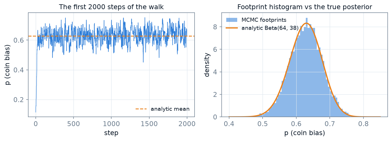
The trace on the left is worth staring at. The first ~50 steps are the walker hiking in from its bad starting point — that transient is called burn-in, and we throw it away because those early footprints reflect where the chain started, not where the probability is. Everything after is the stationary wander that maps the posterior.
Try it yourself: what does the prior do?
The code above uses a flat prior. Suppose a colleague insists the coin is nearly fair. Encode that belief as a Beta(20, 20) prior by adding its log-density to the log-posterior:
def log_post(p):
    if p <= 0.0 or p >= 1.0:
        return -np.inf
    log_prior = 19 * np.log(p) + 19 * np.log(1.0 - p)   # Beta(20, 20)
    return HEADS * np.log(p) + (N - HEADS) * np.log(1.0 - p) + log_prior
Re-run the sampler. You should see the posterior mean pulled from ~0.63 toward 0.5 (the analytic answer becomes Beta(83, 57), mean $83/140 \approx 0.593$) — the data and the prior negotiating. This is the whole Bayesian machinery working in five lines, and exactly how a geophysical prior (e.g., “velocities increase with depth”) reshapes an inversion.
Now the real thing: locating an earthquake
Time to give the sampler a seismological job — the same problem NonLinLoc solves, small enough to grid, so we can trust what the sampler shows us. An earthquake happens at an unknown epicenter $(x, y)$ at unknown origin time $t_0$. Eight stations record P arrivals. With a constant velocity $v$, the forward model is just geometry:
\[t_i^{\mathrm{pred}} = t_0 + \frac{\sqrt{(x_i - x)^2 + (y_i - y)^2}}{v}\]We manufacture a synthetic truth so we can check the answer: epicenter at $(42, 58)$ km, $t_0 = 10$ s, $v = 6$ km/s, and Gaussian pick noise with $\sigma = 0.1$ s.
import numpy as np

rng = np.random.default_rng(7)

stations = np.array([
    [12.0, 15.0], [85.0, 10.0], [90.0, 80.0], [10.0, 85.0],
    [50.0,  5.0], [95.0, 45.0], [45.0, 95.0], [ 5.0, 50.0],
])
TRUE  = np.array([42.0, 58.0, 10.0])   # x (km), y (km), t0 (s)
V     = 6.0                            # km/s
SIGMA = 0.10                           # s, pick uncertainty

def travel_times(x, y, t0):
    d = np.sqrt((stations[:, 0] - x)**2 + (stations[:, 1] - y)**2)
    return t0 + d / V

t_obs = travel_times(*TRUE) + SIGMA * rng.standard_normal(len(stations))
The log-posterior is a Gaussian log-likelihood plus a uniform prior box (any model outside the box gets $-\infty$, i.e., the walker refuses to step outside the survey area):
def log_post(m):
    x, y, t0 = m
    if not (0 <= x <= 100 and 0 <= y <= 100 and 0 <= t0 <= 20):
        return -np.inf                        # uniform prior box
    r = t_obs - travel_times(x, y, t0)
    return -0.5 * np.sum((r / SIGMA)**2)
And the sampler is — this is the point — the same twenty lines as the coin, only walking in three dimensions now:
def run_chain(prop_scale, n_steps=60000, start=(90.0, 15.0, 2.0), seed=7):
    rng = np.random.default_rng(seed)
    m = np.array(start)
    lp = log_post(m)
    chain = np.empty((n_steps, 3))
    accepted = 0
    for i in range(n_steps):
        prop = m + prop_scale * rng.standard_normal(3)
        lp_prop = log_post(prop)
        if np.log(rng.uniform()) < lp_prop - lp:
            m, lp = prop, lp_prop
            accepted += 1
        chain[i] = m
    return chain, accepted / n_steps

chain, acc = run_chain(np.array([0.4, 0.4, 0.05]))   # km, km, s
post = chain[5000:]                                  # drop burn-in
print(acc, post.mean(axis=0), post.std(axis=0))
We deliberately start the chain far from the truth, at $(90, 15)$ km with $t_0 = 2$ s. Watch it find the earthquake:
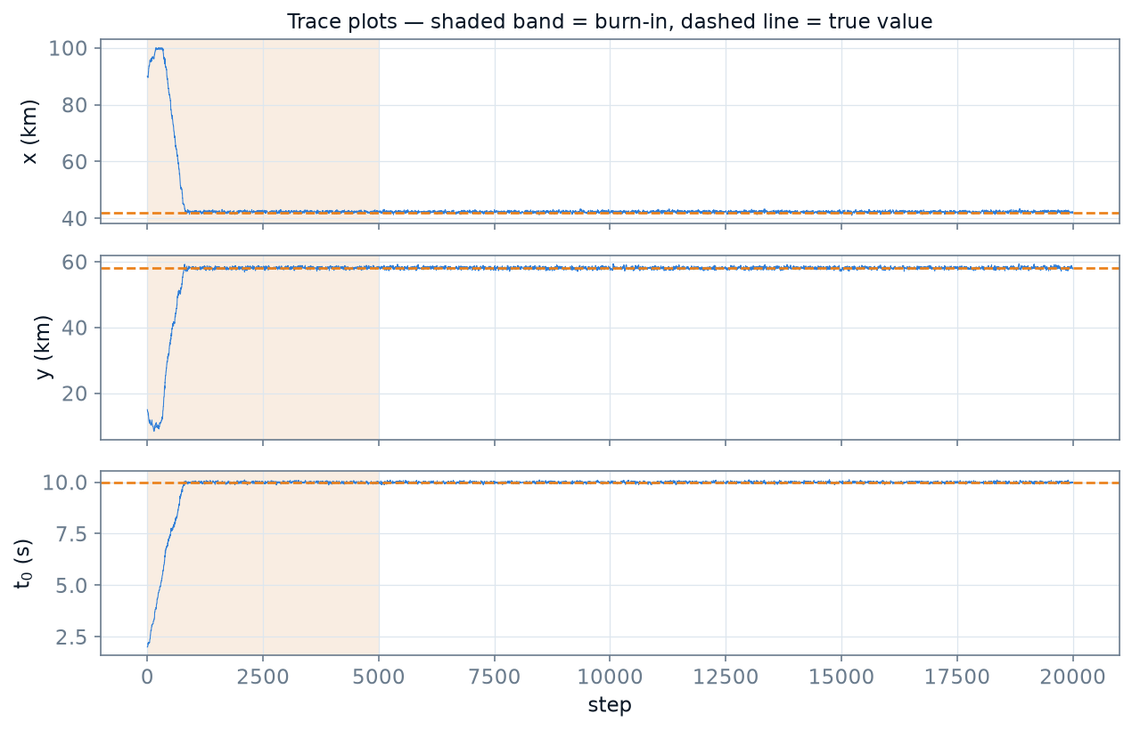
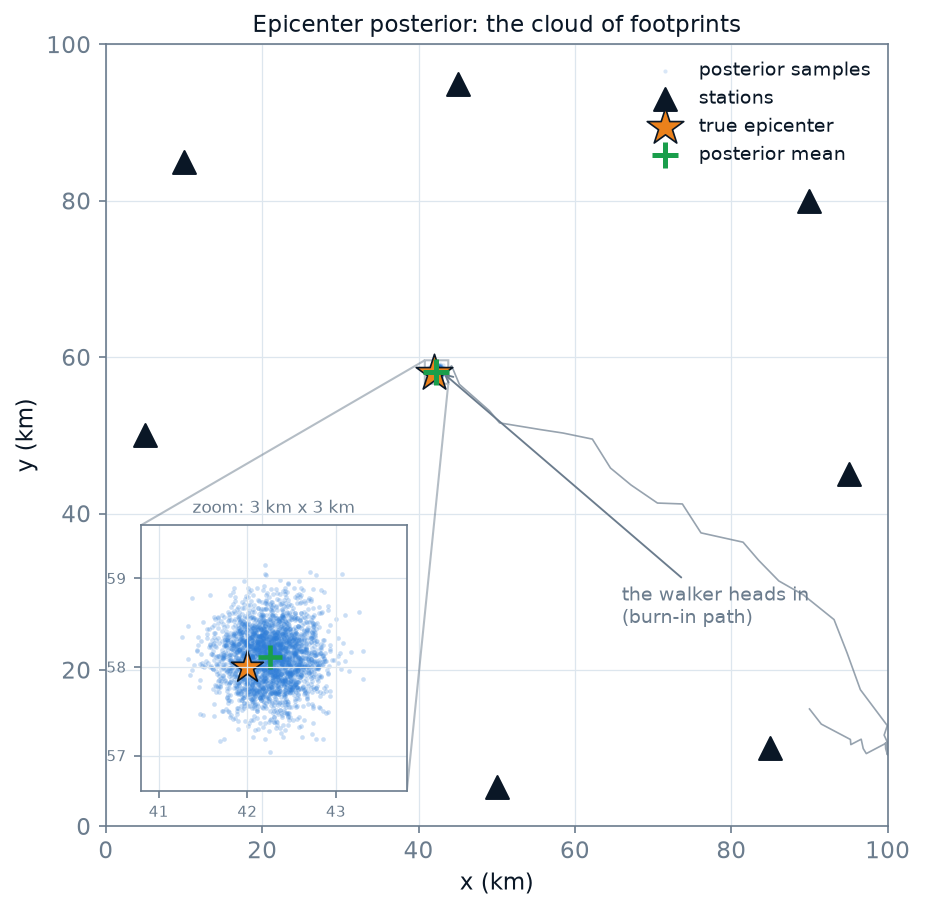
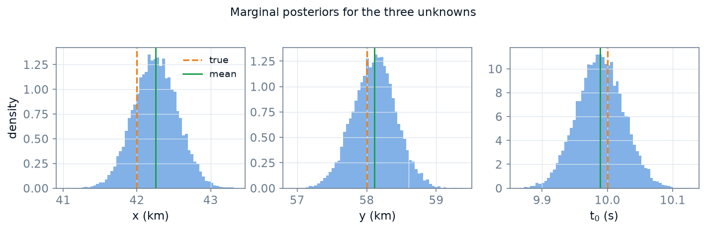
The numbers, against the truth we manufactured:
| Parameter | True | Posterior mean ± std | 95% credible interval |
|---|---|---|---|
| $x$ (km) | 42.0 | 42.25 ± 0.30 | [41.69, 42.83] |
| $y$ (km) | 58.0 | 58.11 ± 0.31 | [57.50, 58.72] |
| $t_0$ (s) | 10.0 | 9.99 ± 0.04 | [9.92, 10.06] |
The true values sit inside the credible intervals, and the posterior mean misses the truth by a fraction of the uncertainty — which is precisely what “the uncertainty is honest” means. Note what we got for free: no derivatives, no linearization, no starting-model sensitivity, and full marginal distributions, from twenty lines of numpy. This is the Metropolis–Gibbs engine inside NonLinLoc (LOCSEARCH MET), stripped to its skeleton — and where NonLinLoc’s oct-tree wins for a 3-parameter hypocenter, the MCMC walk is the tool that keeps working when the parameter count climbs into the tens or hundreds.
Same sampler, any problem
Nothing in the sampler knows about earthquakes. To invert gravity data, receiver functions, or age–depth curves instead, you swap one function — log_post — and the walk does the rest. The forward physics and the sampling machinery are completely decoupled.
How to know the walk went well
MCMC’s honesty depends on the chain actually exploring. Three checks are non-negotiable:
1. Look at the trace plots. A healthy trace looks like a “fuzzy caterpillar” (as in the figures above): rapid fluctuation around a stable level. A trace that drifts, or sits flat for long stretches, has not converged. Always discard the burn-in before computing statistics.
2. Watch the acceptance rate — it’s your step-size dial. When I first ran the earthquake example with steps of 1.5 km, the acceptance rate was 0.03: the posterior is only ~0.3 km wide, so nearly every 1.5 km proposal leapt off the peak and was rejected — the chain stood still 97% of the time. Shrinking the steps to 0.4 km brought acceptance to 0.32, and the chain mixed beautifully. The two failure modes are symmetric:
- Steps too large → almost everything rejected → the chain freezes in place.
- Steps too small → almost everything accepted → the chain inches along, taking ages to cross the posterior.
A rule of thumb many practitioners use: aim for acceptance somewhere around 20–50% for a random-walk sampler, then confirm with the traces.
3. Run multiple chains. Start several walkers from very different points; after burn-in, their histograms must agree. If they don’t, at least one chain is stuck in a local mode — and no single-chain diagnostic would ever have told you.
A stuck chain looks converged: its trace is beautifully stable, because it isn’t going anywhere. Stability of one chain is necessary but never sufficient — only agreement between independent chains (or physics telling you the posterior has one mode) rules out entrapment.
Your chain accepts only 3% of its proposals. What is the most likely diagnosis?
Where MCMC shows up in the geosciences
Once you see inverse problems as posteriors-to-be-sampled, MCMC shows up everywhere. The framework of treating the inverse problem’s solution as the sampled ensemble goes back to Mosegaard & Tarantola [3], and Sambridge & Mosegaard’s review [4] is still the best map of the territory for geophysicists. A few landmarks:
- Seismic tomography and receiver functions — including transdimensional samplers, where the number of model layers or cells is itself unknown and the chain jumps between dimensions (reversible-jump MCMC) [5]. The walker doesn’t just explore one landscape; it can step between landscapes of different sizes.
- Earthquake location — the Metropolis–Gibbs search engine in NonLinLoc is exactly the walk we coded above, wrapped in production machinery.
- Age–depth modeling and geochronology — sampling chronologies consistent with radiometric dates, so every derived rate carries an honest uncertainty.
- Anywhere the model has more parameters than you can grid — which, past three or four, is everywhere.
Where to go next
- Related posts here: Understanding the Metropolis–Hastings algorithm digs into the algorithm’s formal details (proposal asymmetry, the Hastings correction) that I skipped; the NonLinLoc post shows a production-grade probabilistic locator; and Monte Carlo methods and the earthquake location problem covers the plain (non-Markov) Monte Carlo baseline.
- Production samplers: for real research, use a battle-tested library rather than hand-rolled Metropolis — emcee (the affine-invariant ensemble sampler beloved in astro/geophysics) or PyMC (full probabilistic programming with modern gradient-based samplers). Your hand-rolled walker is for understanding; theirs are for publishing.
References
- Equation of State Calculations by Fast Computing Machines — Metropolis, Rosenbluth, Rosenbluth, Teller & Teller, 1953, The Journal of Chemical Physics.
- Monte Carlo sampling methods using Markov chains and their applications — Hastings, 1970, Biometrika.
- Monte Carlo sampling of solutions to inverse problems — Mosegaard & Tarantola, 1995, Journal of Geophysical Research: Solid Earth.
- Monte Carlo methods in geophysical inverse problems — Sambridge & Mosegaard, 2002, Reviews of Geophysics.
- Seismic tomography with the reversible jump algorithm — Bodin & Sambridge, 2009, Geophysical Journal International.
Disclaimer of liability
The information provided by the Earth Inversion is made available for educational purposes only.
Whilst we endeavor to keep the information up-to-date and correct. Earth Inversion makes no representations or warranties of any kind, express or implied about the completeness, accuracy, reliability, suitability or availability with respect to the website or the information, products, services or related graphics content on the website for any purpose.
UNDER NO CIRCUMSTANCE SHALL WE HAVE ANY LIABILITY TO YOU FOR ANY LOSS OR DAMAGE OF ANY KIND INCURRED AS A RESULT OF THE USE OF THE SITE OR RELIANCE ON ANY INFORMATION PROVIDED ON THE SITE. ANY RELIANCE YOU PLACED ON SUCH MATERIAL IS THEREFORE STRICTLY AT YOUR OWN RISK.
Leave a comment