How to plot earthquakes data on a three-dimensional topographic map

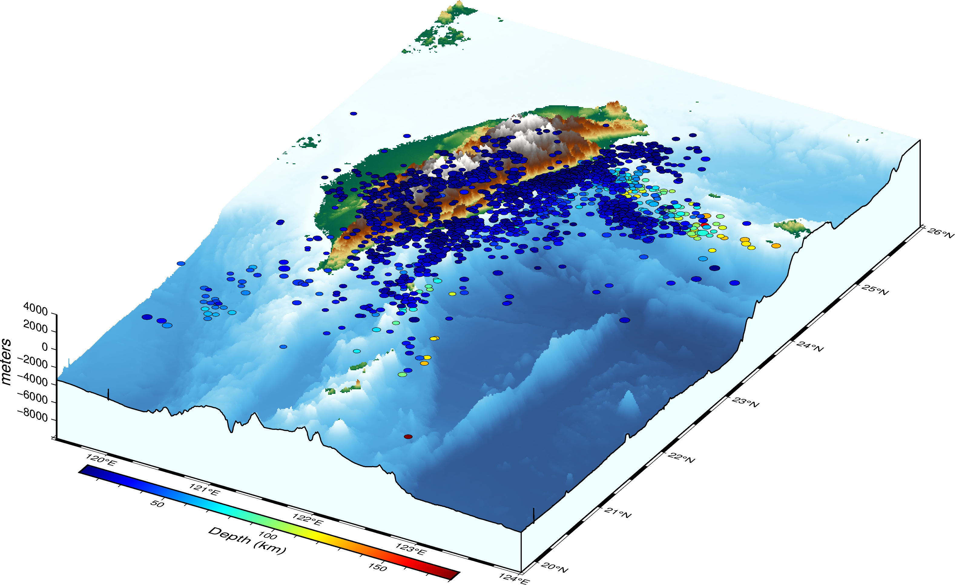
A flat map tells you where earthquakes happen; a three-dimensional map lets you see them hang beneath the topography, so the tie between seismicity and tectonic structure jumps out. Continuing our previous post on overlaying earthquake locations on a 2-D topographic map, this time we drape the events over a 3-D relief surface with PyGMT. The base map is built just like the one in our 3-D perspective map of Taiwan post.

Read the data file

Taiwan is located at a compressive tectonic boundary between the Eurasian Plate and the Philippine Sea Plate. The island straddles the compressional plate boundary between the Eurasian Plate to the west and the north and the Philippine Sea Plate to the east and south. The present convergence rate is about 7 cm/year in a NW-SE direction.

The data for this post was downloaded from Central Weather Administration of Taiwan (formerly the Central Weather Bureau, renamed in September 2023), and saved as evtlist.dat. The dataset contains 2317 events with the date range from 1995-07-05 to 2019-12-16. The depth of the events ranges from 11-180 km, and magnitude (Mw) from 3.0-7.1.

We can read the tabular data using pandas’ read_csv method.

import pandas as pd
# dataformat: 1 1995-07-05 17:33:48.600 24.8313 122.1158 27 4.87
data = pd.read_csv('evtlist.dat', names=['SN','year','time','latitude','longitude','depth_km','magnitude'], delimiter='\s+')

Load the topographic data

We load the topographic data directly using the PyGMT load_earth_relief method. The PyGMT will download the specified resolution of the topographic data locally.

minlon, maxlon = 119.5, 124.0
minlat, maxlat = 19.8, 26.0
# Load sample earth relief data
grid = pygmt.datasets.load_earth_relief(resolution="03s", region=[minlon, maxlon, minlat, maxlat])

Define three-dimensional perspective

We first specify the cpt files for the topographic colors, and then we specify the three-dimensional perspective view. The view is set to have the azimuth and elevation angle of the viewpoint to be 150 and 30 degrees. The cover type of the grid is taken as “surface”. The other options are mesh, waterfall, image, etc. See the pygmt.Figure.grdview for details.

We define the region by the bounds of latitudes, longitudes and depths. The projection was taken to be “Mercator” with width of 15cm. The vertical height was taken to be 4cm.

pygmt.makecpt(
        cmap='geo',
        series=f'-{maxdep}/4000/100',
        continuous=True
    )
fig = pygmt.Figure()
fig.grdview(
    grid=grid,
    region=[minlon, maxlon, minlat, maxlat, -maxdep, 4000],
    perspective=[150, 30],
    frame=frame,
    projection="M15c",
    zsize="4c",
    surftype="i",
    plane=f"-{maxdep}+gazure",
    shading=0,
    # Set the contour pen thickness to "1p"
    contourpen="1p",
)

Plot the data on a topographic map

Since the depths of the event ranges up to 180 km, we had to constrain it to show it within the range of our chosen maximum depth for the three-dimensional map. We project the depths in the range of 0 to the maximum depth of the displayed topography.

Another good choice for displaying the actual depth for each earthquake events is displaying on a cross-sectional map. The advantage of displaying the events on the topographic map is understanding its relation with the tectonics (topography or bathymetry).

depthData = data.depth_km.values
depthData = maxdep*(depthData - data.depth_km.min())/(data.depth_km.max()-data.depth_km.min()) #normalize the depth to the maximum of maxdep

# colorbar colormap
pygmt.makecpt(cmap="jet", series=[
              depthData.min(), depthData.max()])

fig.plot3d(
    x=data.longitude,
    y=data.latitude,
    z=-1*depthData,
    size=0.05*data.magnitude, #scale the magnitude
    color=depthData,
    cmap=True,
    style="cc",
    pen="black",
    perspective=True,
)

Note the two roles depth plays here: it is rescaled to fit the vertical extent of the plot (so the symbols sit inside the box), and — via a second makecpt below — it drives the color of each symbol. Symbol size (0.05*data.magnitude) encodes magnitude, so a single glance conveys location, depth, and size at once.

Add colorbar to the figure

At last, we can add the colorbar to show the values of actual depths of the event. This is why we call makecpt a second time with the real depth range (data.depth_km, not the rescaled values) — the bar must read in true kilometres even though the symbol positions were normalized.

pygmt.makecpt(cmap="jet", series=[
              data.depth_km.min(), data.depth_km.max()])
fig.colorbar(frame='af+l"Depth (km)"', perspective=True,)

Complete script

Recap

• Layered, single-perspective assembly. grdview → plot3d → colorbar, all sharing perspective=[150, 30] and the same 3-D region, is what makes points line up with the terrain.
• Depth does double duty. Rescale it to fit the z-axis (positions inside the box) and map it to a colormap (symbol color); magnitude maps to symbol size.
• Colorbar shows true depth. Run makecpt once on normalized depths for plotting, and again on the real km values for the bar.
• Watch the API names. On PyGMT ≥ v0.8, use fill= (not color=) in plot3d and contour_pen (not contourpen) in grdview.

Where to go next

• 2-D version of this map: Plot earthquake data on a topographic map
• The 3-D base map, step by step: Three-dimensional perspective map of Taiwan using GMT and PyGMT
• PyGMT grdview API: pygmt.org/dev/api/generated/pygmt.Figure.grdview.html
• PyGMT plot3d API: pygmt.org/dev/api/generated/pygmt.Figure.plot3d.html

References

1. Quantifying the seismicity on Taiwan — Yi-Hsuan Wu, Chien-Chih Chen, Donald L. Turcotte, John B. Rundle, 2013, Geophysical Journal International, 194(1), 465–469.