Estimation of the degrees of freedom of time series in Python (codes included)
Introduction
The correlation between two (real) stochastic processes A and B, which are sampled as two (real) time series, A(t) and B(t) can be written as
\[\rho (\tau) = \sum_i A(t_i-\tau) B(t_i)/[\sum_i A(t_i)^2 \sum_i B(t_i)^2]^{(1/2)}\]A dimensionless number between 1 and −1 (the Cauchy‐Schwarz inequality), the correlation \(\rho\) by its face value alone does not dictate whether or not the correlation in question is significant unless the degrees of freedom (DOF) of the processes, which signifies the information content (or entropy), is also specified.
As discussed in the previous post, two time series with predominant linear trends (very low DOF) can have a very high \(\rho\), which can hardly be construed as evidence for a meaningful physical relationship.
A relatively high \(\rho\) for low DOF may be less significant than a relatively low \(\rho\) at high DOF and vice versa.
Given the DOF of processes A and B, what is the probability at which the obtained \(\rho\) can reject the null hypothesis that A and B are actually uncorrelated? The probability \(P_c\) for the correlation value to exceed a certain |\(\rho\)| (between 0 and 1) for random samples with DOF = ν is given by \(P_c(\rho; \nu) = 1/\sqrt(\pi) \frac{\Gamma[(\nu + 1)/2]}{\Gamma (\nu / 2)} \int_{|\rho|}^{1} (1-x**2)^{(\nu - 2)/2} dx\) where \(Γ(z) = ∫_0^\inf x^{z−1} e^{−x} dx\) is the Gamma function. The significance level is 2\(P_c\), accounting for both positive and negative ρ values, and the confidence level is 1‐2\(P_c\), for given \(\nu\).
What is degrees of freedom?
It is intuitively unwise to both estimate the parameters and perform the test from the same set of data without somehow compensating for the double use of observations. The compensation is done by considering a quantity called degrees of freedom (DOF).
The degrees of freedom may be defined as the number of observations in a sample minus the number of parameters estimated from the sample. In other words, the DOFare the number of observations in excess of those necessary to estimate the parameters of the distribution. It can also be seen as the number of independent comparisons that can be made between the observations in the estimating samples. In most of the elementary problems, it is just one less than the total number of observations. For instance, if we have three observations - A, B, C. The possible comparisons between these three are A->B, A->C and C->B. But if we know any two of them, we automatically know the relationships between the third.
How to find the degrees of freedom of time series?
For a Gaussian (white) time series with N independent numbers, the DOF is equal to \(N-2\); the loss of 2 degrees of freedom is to account for the specification of the mean and standard deviation. However, the DOF for nonwhite time series is smaller than \(N-2\) given that the sampled values are not entirely independent of each other. There are several schemes for the estimation of DOF (for details see Wang et. al., 1999).
We need to apply several statistical analysis of time series to understand variability, regular and irregular oscillations, characteristics of these oscillations,and the physical processes that give rise to each of these oscillations.
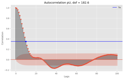
Autocorrelation can be used to estimate the dominant periods in the time series. The autocovariance is the covariance of a variable with itself at some other time, measured by a time lag (or lead) \(\tau\). The typical autocorrelation function tells us that data points in a time series are not independent. For a time series of red noise, it has been suggested that the degree of freedom can be determined as following (Panofsky and Brier, 1958):
\[DOF = \frac{N \Delta t}{2T_e}\]Here \(T_e\) is the e-folding decay time of autocorrelation (where autocorrelation drops to \(1/e\)). \(\Delta t\) is the time interval between data.
We can obtain an estimate of the degrees of freedom of a time series.
from statsmodels.tsa.stattools import acf
from statsmodels.graphics import tsaplots
import matplotlib.pyplot as plt
import numpy as np
from time_series import pU
#ref: Panofsky and Brier 1968


for i,val in enumerate(acf(pU)):
    if val < 1/np.exp(1):
        print(i,val)
        Te = i
        val_Te = val
        break
dof = (len(pU)*1)/(2*Te)
print(f"Num degrees of freedom is {dof}")
fig = tsaplots.plot_acf(pU, lags=100,alpha=0.05)
plt.plot(Te,val_Te,'bo')
plt.axhline(val_Te,color='b',label='Te')
plt.legend(loc=0)
plt.xlabel('Lags')
plt.ylabel('Correlation')
plt.title(f'Autocorrelation pU, dof = {dof}',fontsize=14)
plt.savefig(f'Autocorr_pU.png',bbox_inches='tight')
plt.close('all')
References:
- Chao, B. F., and C. H. Chung (2019), On Estimating the Cross Correlation and Least Squares Fit of One Data Set to Another With Time Shift, Earth and Space Science, 6(8), 1409–1415, doi:10.1029/2018EA000548.
- Wang, X., S. S. Shen, X. Wang, and S. S. Shen (1999), Estimation of Spatial Degrees of Freedom of a Climate Field, http://dx.doi.org/10.1175/1520-0442(1999)012<1280:EOSDOF>2.0.CO;2, 12(5), 1280–1291, doi:10.1175/1520-0442(1999)012<1280:EOSDOF>2.0.CO;2.
- Panofsky, H.A. and Brier, G.W., 1958. Some applications of statistics to meteorology. Mineral Industries Extension Services, College of Mineral Industries, Pennsylvania State University.
- Davis, J., & Sampson, R. (1986). Statistics and data analysis in geology. Retrieved from https://www.academia.edu/download/6413890/clarifyeq4-81.pdf
Disclaimer of liability
The information provided by the Earth Inversion is made available for educational purposes only.
Whilst we endeavor to keep the information up-to-date and correct. Earth Inversion makes no representations or warranties of any kind, express or implied about the completeness, accuracy, reliability, suitability or availability with respect to the website or the information, products, services or related graphics content on the website for any purpose.
UNDER NO CIRCUMSTANCE SHALL WE HAVE ANY LIABILITY TO YOU FOR ANY LOSS OR DAMAGE OF ANY KIND INCURRED AS A RESULT OF THE USE OF THE SITE OR RELIANCE ON ANY INFORMATION PROVIDED ON THE SITE. ANY RELIANCE YOU PLACED ON SUCH MATERIAL IS THEREFORE STRICTLY AT YOUR OWN RISK.
Leave a comment