GMT Advanced Tutorial, Part II (codes included)
Continuation of Part I
Introduction
For basic tutorial, please visit here.
This tutorial consists of Bash script files to run the GMT. The data files required to run the scripts can be downloaded from here. Most codes are minor modifications of the GMT historical collections.
Bash Scripts
Following scripts are obtained mostly from GMT website and is being presented here with slight modifications, if any.
Missing data: Gridding and clipping
![]()
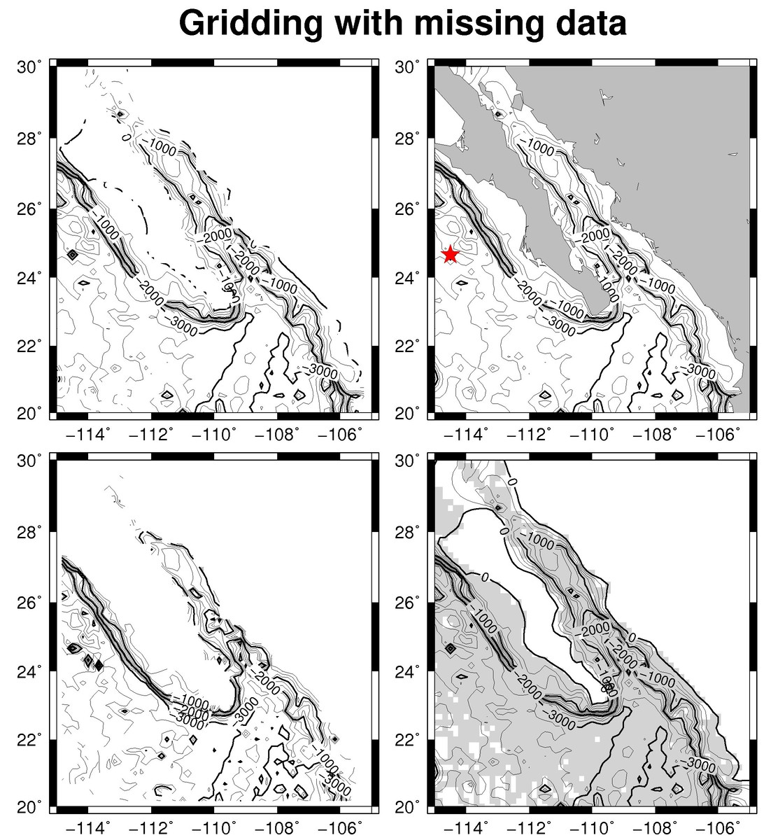
We first convert a large ASCII file to binary with gmtconvert since the binary file will read and process much faster. Our lower left plot illustrates the results of gridding using a nearest neighbor technique (nearneighbor) which is a local method: No output is given where there are no data.
Next (lower right), we use a minimum curvature technique (surface) which is a global method. Hence, the contours cover the entire map although the data are only available for portions of the area (indicated by the gray areas plotted using psmask). The top left scenario illustrates how we can create a clip path (using psmask) based on the data coverage to eliminate contours outside the constrained area.
Finally (top right) we simply employ pscoast to overlay gray land masses to cover up the unwanted contours, and end by plotting a star at the deepest point on the map with psxy.
#!/bin/bash

ctr="-Xc -Yc"
for i in 1
do
	fig[i]="Figures/GMT_example8-${i}.ps"
done

gmt convert Data/ship.xyz -bo > ship.b #-bo selects native binary output
#
region=`gmt info ship.b -I1 -bi3d` #-bi3d: selects native binary input, 3 number of columns, 8 byte double precision float
# echo $region
gmt nearneighbor $region -I10m -S40k -Gship.nc ship.b -bi #-I10m-> grid spacing 10 arc minutes,
#-S40k : 40km search radius
#-Goutput_grdfile

gmt grdcontour ship.nc -JM3i -P -B2 -BWSne -C250 -A1000 -Gd2i -Y2i -K> ${fig[1]}
#-Gd2i: 2i distance between labels in the plot
# #
gmt blockmedian $region -I10m ship.b -b3d > ship_10m.b
gmt surface $region -I10m ship_10m.b -Gship.nc -bi
gmt psmask $region -I10m ship.b -J -O -K -T -Glightgray -bi3d -X3.6i >> ${fig[1]}
gmt grdcontour ship.nc -J -B -C250 -L-8000/0 -A1000 -Gd2i -O -K >> ${fig[1]}
# #
gmt psmask $region -I10m ship_10m.b -bi3d -J -B -O -K -X-3.6i -Y3.75i >> ${fig[1]}
gmt grdcontour ship.nc -J -C250 -A1000 -L-8000/0 -Gd2i -O -K >> ${fig[1]}
gmt psmask -C -O -K >> ${fig[1]}
# #
gmt grdclip ship.nc -Sa-1/NaN -Gship_clipped.nc
gmt grdcontour ship_clipped.nc -J -B -C250 -A1000 -L-8000/0 -Gd2i -O -K -X3.6i >> ${fig[1]}
gmt pscoast $region -J -O -K -Ggray -Wthinnest >> ${fig[1]}
gmt grdinfo -C -M ship.nc | gmt psxy -R -J -O -K -Sa0.15i -Wthick,red -Gred -i11,12 >> ${fig[1]}
echo "-0.3 3.6 Gridding with missing data" | gmt pstext -R0/3/0/4 -Jx1i \
	-F+f24p,Helvetica-Bold+jCB -O -N >> ${fig[1]}

rm -f ship.b ship_10m.b ship.nc ship_clipped.nc gmt*
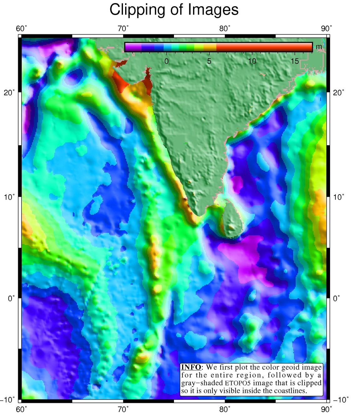
Clipping of map along coastlines
![]()
#!/bin/bash

ctr="-Xc -Yc"

for i in 1
do
	fig[i]="Figures/GMT_example9-${i}.ps"
done
# First generate geoid image w/ shading
gmt grd2cpt Data/india_geoid.nc -Crainbow > geoid.cpt
gmt grdgradient Data/india_geoid.nc -Nt1 -A45 -Gindia_geoid_i.nc
gmt grdimage Data/india_geoid.nc -Iindia_geoid_i.nc -JM6.5i -Cgeoid.cpt -P -K $ctr > ${fig[1]}

# Then use gmt pscoast to initiate clip path for land

gmt pscoast -RData/india_geoid.nc -J -O -K -Dl -Gc >> ${fig[1]}

# Now generate topography image w/shading

gmt makecpt -Ctopo -T-10000/10000 -N > shade.cpt
gmt grdgradient Data/india_topo.nc -Nt1 -A45 -Gindia_topo_i.nc
gmt grdimage Data/india_topo.nc -Iindia_topo_i.nc -J -Cshade.cpt -O -K >> ${fig[1]}

# Finally undo clipping and overlay basemap

gmt pscoast -R -J -O -K -Q -B10f5 -B+t"Clipping of Images" >> ${fig[1]}

# Put a color legend on top of the land mask

gmt psscale -DjTR+o0.3i/0.1i+w4i/0.2i+h -R -J -Cgeoid.cpt -Bx5f1 -By+lm -I -O -K >> ${fig[1]}

# Add a text paragraph

gmt pstext -R -J -O -M -Gwhite -Wthinner -TO -D-0.1i/0.1i -F+f12,Times-Roman+jRB >> ${fig[1]} << END
> 90 -10 12p 3i j
@_@%5%INFO@%%@_:  We first plot the color geoid image
for the entire region, followed by a gray-shaded @#etopo5@#
image that is clipped so it is only visible inside the coastlines.
END

# Clean up
rm -f geoid.cpt shade.cpt *_i.nc
Plot custom symbols
![]()
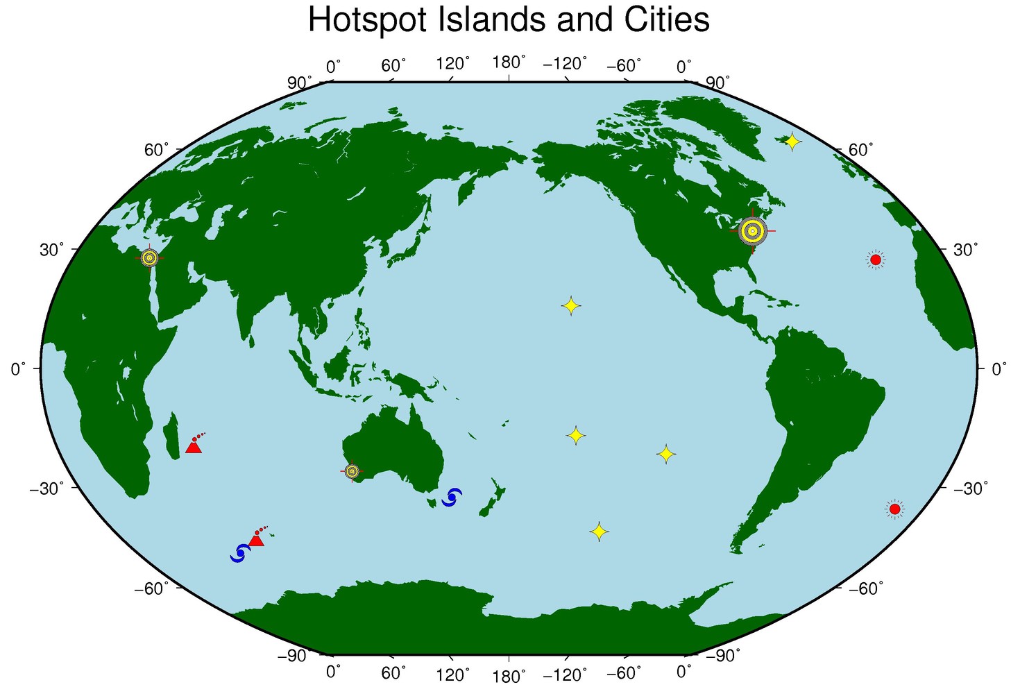
Plot a world-map with volcano symbols of different sizes
on top given locations and sizes in hotspots.d
#!/bin/bash
ctr="-Xc -Yc"

for i in 1
do
	fig[i]="Figures/GMT_example10-${i}.ps"
done

cat > hotspots1.d << END
55.5	-21.0	0.5
63.0	-49.0	0.5
END
cat > hotspots2.d << END
-12.0	-37.0	0.5
-28.5	29.34	0.5
END
cat > hotspots3.d << END
48.4	-53.4	0.5
155.5	-40.4	0.5
END
cat > hotspots4.d << END
-155.5	19.6	0.5
-138.1	-50.9	0.5
-153.5	-21.0	0.5
-116.7	-26.3	0.5
-16.5	64.4	0.5
END
gmt pscoast -Rg -JR9i -Bx60 -By30 -B+t"Hotspot Islands and Cities" -Gdarkgreen -Slightblue \
	-Dc -A5000 -K > ${fig[1]}

gmt psxy -R -J hotspots1.d -Skvolcano -O -K -Wthinnest -Gred >> ${fig[1]}
gmt psxy -R -J hotspots2.d -SkCustomSymbols/sun -O -K -Wthinnest -Gred >> ${fig[1]}
gmt psxy -R -J hotspots3.d -SkCustomSymbols/hurricane -O -K -Wthinnest -Gblue >> ${fig[1]}
gmt psxy -R -J hotspots4.d -SkCustomSymbols/astroid -O -K -Wthinnest -Gyellow >> ${fig[1]}

# Overlay a few bullseyes at NY, Cairo, and Perth

cat > cities.d << END
286	40.45	0.8
31.15	30.03	0.5
115.49	-31.58	0.4
END

gmt psxy -R -J cities.d -SkCustomSymbols/bullseye -O >> ${fig[1]}

rm -f hotspots*.d cities.d gmt*
Plot of last 7 days of seismicity from USGS
![]()
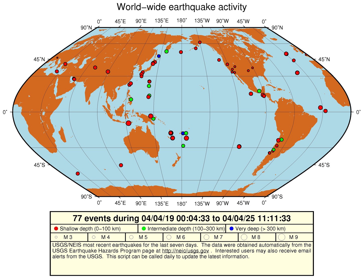
Get the data (-q quietly) from USGS using the wget (comment out in case your system does not have wget or curl)
wget http://neic.usgs.gov/neis/gis/bulletin.asc -q -O Data/neic_quakes.d
curl http://neic.usgs.gov/neis/gis/bulletin.asc -s > Data/neic_quakes.d
#!/bin/bash

ctr="-Xc -Yc"

for i in 1
do
	fig[i]="Figures/GMT_example11-${i}.ps"
done
gmt set FONT_ANNOT_PRIMARY 10p FONT_TITLE 18p FORMAT_GEO_MAP ddd:mm:ssF


# Count the number of events (to be used in title later. one less due to header)
n=`cat Data/neic_quakes.d | wc -l`
n=`expr $n - 1`

# Pull out the first and last timestamp to use in legend title
first=`sed -n 2p Data/neic_quakes.d | awk -F, '{printf "%s %s\n", $1, $2}'` #sed print the 2nd line
last=`sed -n '$p' Data/neic_quakes.d | awk -F, '{printf "%s %s\n", $1, $2}'` #sed print the last line
# Assign a string that contains the current user @ the current computer node.
# Note that two @@ is needed to print a single @ in gmt pstext:


# Start plotting. First lay down map, then plot quakes with size = magintude/50":

gmt pscoast -Rg -JK180/9i -B45g30 -B+t"World-wide earthquake activity" -Gchocolate -Slightblue \
	-Dc -A1000 -Y2.75i -K > ${fig[1]}
awk -F, '{ print $4, $3, $6, $5*0.02}' Data/neic_quakes.d \
	| gmt psxy -R -JK -O  -CCPTs/quakes.cpt -Sci -Wthin -h -K >> ${fig[1]}
# Create legend input file for NEIS quake plot

cat > neis.legend << END
H 16 1 $n events during $first to $last
D 0 1p
N 3
V 0 1p
S 0.1i c 0.1i red 0.25p 0.2i Shallow depth (0-100 km)
S 0.1i c 0.1i green 0.25p 0.2i Intermediate depth (100-300 km)
S 0.1i c 0.1i blue 0.25p 0.2i Very deep (> 300 km)
D 0 1p
V 0 1p
N 7
V 0 1p
S 0.1i c 0.06i - 0.25p 0.3i M 3
S 0.1i c 0.08i - 0.25p 0.3i M 4
S 0.1i c 0.10i - 0.25p 0.3i M 5
S 0.1i c 0.12i - 0.25p 0.3i M 6
S 0.1i c 0.14i - 0.25p 0.3i M 7
S 0.1i c 0.16i - 0.25p 0.3i M 8
S 0.1i c 0.18i - 0.25p 0.3i M 9
D 0 1p
V 0 1p
N 1
END

# Put together a reasonable legend text, and add logo and user's name:

cat << END >> neis.legend
G 0.25l
P
T USGS/NEIS most recent earthquakes for the last seven days.  The data were
T obtained automatically from the USGS Earthquake Hazards Program page at
T @_http://neic/usgs.gov @_.  Interested users may also receive email alerts
T from the USGS.
T This script can be called daily to update the latest information.
G 0.4i
G -0.3i
L 12 6 LB
END

# OK, now we can actually run gmt pslegend.  We center the legend below the map.
# Trial and error shows that 1.7i is a good legend height:

gmt pslegend -DJBC+o0/0.4i+w7i/1.7i -R -J -O -F+p+glightyellow neis.legend  >> ${fig[1]}

# Clean up after ourselves:

rm -f neis.* gmt.conf
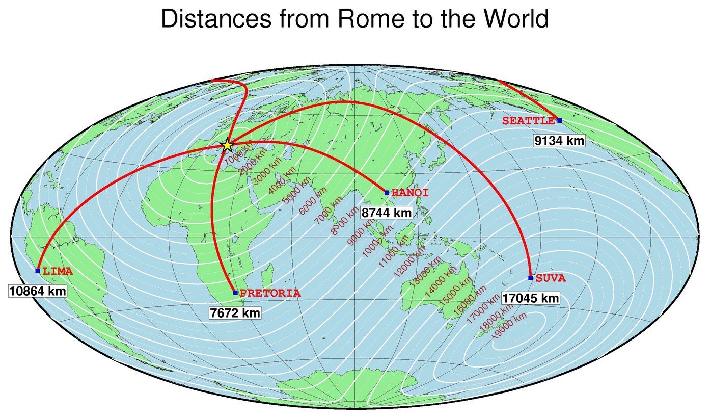
Plot of shortest path between two places
![]()
#!/bin/bash

ctr="-Xc -Yc"

for i in 1
do
	fig[i]="Figures/GMT_example12-${i}.ps"
done
# Position and name of central point:

lon=12.50
lat=41.99
name="Rome"

# Calculate distances (km) to all points on a global 1x1 grid

gmt grdmath -Rg -I1 $lon $lat SDIST = dist.nc

# Location info for 5 other cities + label justification

cat << END > cities.d
105.87	21.02	HANOI		LM
282.95	-12.1	LIMA		LM
178.42	-18.13	SUVA		LM
237.67	47.58	SEATTLE		RM
28.20	-25.75	PRETORIA	LM
END

gmt pscoast -Rg -JH90/9i -Glightgreen -Slightblue -A1000 -Dc -Bg30 \
	-B+t"Distances from $name to the World" -K -Wthinnest > ${fig[1]}

gmt grdcontour dist.nc -A1000+v+u" km"+fbrown -Glz-/z+ -S8 -C500 -O -K -J \
	-Wathin,white -Wcthinnest,white,- >> ${fig[1]}

# For each of the cities, plot great circle arc to Rome with gmt psxy
gmt psxy -R -J -O -K -Wthickest,red -Fr$lon/$lat cities.d >> ${fig[1]}

# Plot red squares at cities and plot names:
gmt psxy -R -J -O -K -Ss0.2 -Gblue -Wthinnest cities.d >> ${fig[1]}
awk '{print $1, $2, $4, $3}' cities.d | gmt pstext -R -J -O -K -Dj0.15/0 \
	-F+f12p,Courier-Bold,red+j -N >> ${fig[1]}
# Place a yellow star at Rome
echo "$lon $lat" | gmt psxy -R -J -O -K -Sa0.2i -Gyellow -Wthin >> ${fig[1]}

# Sample the distance grid at the cities and use the distance in km for labels

gmt grdtrack -Gdist.nc cities.d \
	| awk '{printf "%s %s %d km\n", $1, $2, int($NF+0.5)}' \
	| gmt pstext -R -J -O -D0/-0.2i -N -Gwhite -W -C0.02i -F+f12p,Helvetica-Bold+jCT >> ${fig[1]}

# Clean up after ourselves:

rm -f cities.d dist.nc
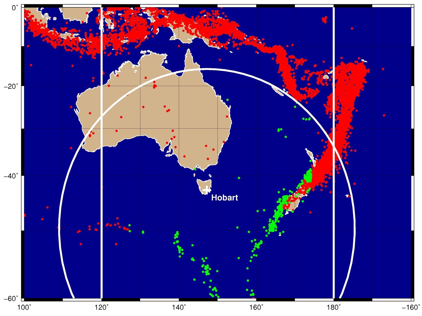
Extract subset of data based on geospatial criteria
![]()
#!/bin/bash


# Highlight oceanic earthquakes within 3000 km of Hobart and > 1000 km from dateline
ctr="-Xc -Yc"

for i in 1
do
	fig[i]="Figures/GMT_example13-${i}.ps"
done


echo "147:13 -42:48 6000" > point.txt
cat << END > dateline.txt
> Our proxy for the dateline
180	0
180	-90
>another line
120 0
120 -90
END
R=`gmt info -I10 Data/oz_quakes.d`
gmt pscoast $R -JM9i -K -Gtan -Sdarkblue -Wthin,white -Dl -A500 -Ba20f10g10 -BWeSn > ${fig[1]}
gmt psxy -R -J -O -K Data/oz_quakes.d -Sc0.05i -Gred >> ${fig[1]}
gmt select Data/oz_quakes.d -L500k/dateline.txt -Nk/s -C3000k/point.txt -fg -R -Il -fo > Data/selected_quakes.txt #long, lat, depth, mag
gmt select Data/oz_quakes.d -L500k/dateline.txt -Nk/s -C3000k/point.txt -fg -R -Il \
	| gmt psxy -R -JM -O -K -Sc0.05i -Ggreen >> ${fig[1]}
#-Nk/s for condition wet areas only
gmt psxy point.txt -R -J -O -K -SE- -Wfat,white >> ${fig[1]}
gmt pstext point.txt -R -J -F+f14p,Helvetica-Bold,white+jLT+tHobart \
	-O -K -D0.1i/-0.1i >> ${fig[1]}
gmt psxy -R -J -O -K point.txt -Wfat,white -S+0.2i >> ${fig[1]}
gmt psxy -R -J -O dateline.txt -Wfat,white -A >> ${fig[1]}
rm -f point.txt dateline.txt
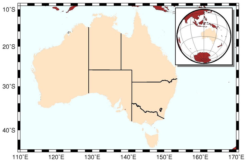
Map inserts
![]()
#!/bin/bash

ctr="-Xc -Yc"

for i in 1 2 3
do
fig[i]="Figures/GMT_example14-\${i}.ps"
done

# Bottom map of Australia

gmt pscoast -R110E/170E/44S/9S -JM6i -P -Baf -BWSne -Wfaint -N2/1p -EAU+gbisque -Gbrown -Sazure1 -Da -K $ctr --FORMAT_GEO_MAP=dddF > ${fig[1]}
gmt psbasemap -R -J -O -K -DjTR+w1.5i+o0.15i/0.1i+stmp -F+gwhite+p1p+c0.1c+s >> ${fig[1]}
read x0 y0 w h < tmp
gmt pscoast -Rg -JG120/30S/$w -Da -Gbrown -A5000 -Bg -Wfaint -EAU+gbisque -O -K -X$x0 -Y$y0 >> ${fig[1]}
gmt psxy -R -J -O -T  -X-${x0} -Y-${y0} >> ${fig[1]}

# Determine size of insert map of Europe

gmt mapproject -R15W/35E/30N/48N -JM2i -W > tmp
read w h < tmp
gmt pscoast -R10W/5E/35N/44N -JM6i -Baf -BWSne -EES+gbisque -Gbrown -Wfaint -N1/1p -Sazure1 -Df -Y4.5i --FORMAT_GEO_MAP=dddF -P -K > ${fig[2]}
gmt psbasemap -R -J -O -K -DjTR+w$w/$h+o0.15i/0.1i+stmp -F+gwhite+p1p+c0.1c+s >> ${fig[2]}
read x0 y0 w h < tmp
gmt pscoast -R15W/35E/30N/48N -JM$w -Da -Gbrown -B0 -EES+gbisque -O -K -X$x0 -Y$y0 --MAP_FRAME_TYPE=plain >> ${fig[2]}
gmt psxy -R -J -O -T -X-${x0} -Y-${y0} >> \${fig[2]}

# Determine size of insert map of Taiwan

twinset="-R100/140/5/40"
gmt mapproject ${twinset} -JM2i -W > tmp
read w h < tmp
gmt pscoast -R117E/124E/20N/28N -JM6i -Baf -BWSne -ETW+gbisque -Gbrown -Wthick -A5000 -N1/1p -Sazure1 -Df --FORMAT_GEO_MAP=dddF -P -K $ctr> ${fig[3]}
gmt psbasemap -R -J -O -K -DjTR+w$w/$h+o0.15i/0.1i+stmp -F+gwhite+p1p+c0.1c+s >> ${fig[3]}
read x0 y0 w h < tmp
gmt pscoast ${twinset} -JM$w -Da -Gbrown -B0 -ETW+gbisque -O -K -X$x0 -Y$y0 --MAP_FRAME_TYPE=plain >> ${fig[3]}
gmt psxy -R -J -O -T -X-${x0} -Y-${y0} >> ${fig[3]}
rm -f tmp
Disclaimer of liability
The information provided by the Earth Inversion is made available for educational purposes only.
Whilst we endeavor to keep the information up-to-date and correct. Earth Inversion makes no representations or warranties of any kind, express or implied about the completeness, accuracy, reliability, suitability or availability with respect to the website or the information, products, services or related graphics content on the website for any purpose.
UNDER NO CIRCUMSTANCE SHALL WE HAVE ANY LIABILITY TO YOU FOR ANY LOSS OR DAMAGE OF ANY KIND INCURRED AS A RESULT OF THE USE OF THE SITE OR RELIANCE ON ANY INFORMATION PROVIDED ON THE SITE. ANY RELIANCE YOU PLACED ON SUCH MATERIAL IS THEREFORE STRICTLY AT YOUR OWN RISK.
Leave a comment